Machine learning is the capability of machines to imitate human behaviour while solving problems. It involves computers using algorithms to find insightful information through an iterative process.

The machine learning process begins with inputing training data in an algorithm of choice. The training data alters the weights and biases within the algorithm, new input data is then fed into the algorithm to make predictions. The predictions are then compared with the actual values to check if the results match, if they dont. The algorithm is retrained until the desired outcome is achieved.

There are two primary areas of machine learning, the supervised and unsupervised learning.

Supervised machine learning uses labeled data from the training data. In this piece, we build and implement supervised algorithms such as linear regression, logistic regression, decision trees, random forest, adaboost, support vector machines, k-nearest neighbors, linear discriminant analysis, and Naive Bayes.
Unsupervised machine learning uses unlabeled data, the trained model tries to search for patterns. We explore two popular unsupervised algorithms namely, principal components analysis and K-means clustering.

Linear Regression: Least Square Method

Given independent variable $x= [1,2,3,4,5]$ and dependent variable $y = [2,4,5,4,5]$ . Using the linear model $y = b + wx$ , we can calculate the slope (w) and the intercept ( $b$ ).

The mean of $\tilde{x}=3$ and $\tilde{y}=4$ , all the regresssion lines must go through their point of interception.

The slope $w = \frac{\sum(x-\tilde{x})(y-\tilde{y})}{\sum(x - \tilde{x})^2} = \frac{6}{10}$

Since $x=3, y=4, w=0.6$ . Intercept $b = y-wx \Rightarrow b=4 - (0.6*3)=2.2$

The regression formula becomes $\hat{y} = 2.2 + .6x$

R Squared

It tells how well a regression formula predicts the actual values, if the actual is very close to the estimates then $R^2 = 1$ . From our x above, we can use $\tilde{y} = 2.2 + .6x$ , with $\tilde{x}=3, \tilde{y}=4$ to estimate the values as follows;

$R^2 = \frac{sum(estimate-mean)}{sum(actual-mean)} = \frac{\sum(\hat{y} - \tilde{y})^2}{\sum(y-\tilde{y})^2} = \frac{[((2.2+(0.6*1) - 4)^2=1.4, 0.36, 0, 0.36, 1.44] = 3.6} {[(2-4)^2=4, 0, 1, 0, 1]=6} = 0.6$

Standard Error of the Estimate

The distance between the actual and the estimated (error). $SE = \sqrt \frac {\sum(estimate-actual)^2}{n-2} = \sqrt{\frac{\sum(\hat{y} - y)^2}{n-2}} = \frac{\sum[(2.2+(0.6*1)-2)^2=.64, 0.36, 1, 0.36, 2.4]}{5-2}= 0.89$

Standard Deviation

The deviation of values of a variable from the mean, $S_y = \sqrt{\frac{\sum(x-\tilde{x})^2}{sample(n-1) \ or \ pop(n)}} = \frac{ \sum([(2-4)^2, (4-4)^2, (5-4)^2, (4-4)^2, (5-4)^2])}{5-1} =1.22$

Correlation

A measure of strength of association between two variables. Where as, regression predicts one variable given another variable.

Pearson's \ r = \frac{ \sum((x-\tilde{x})*(y-\tilde{y}))}{ \sqrt{\sum(x-\tilde{x})^2 * \sum(y-\tilde{y})^2} } = 0.775

0<4<0.19: v.low, 0.2<r<0.39:low, 0.4<r<0.59: moderate, 0.6<r0.79:high, 0.8<r<1: v.high

Implementing Linear Regression in Python

Use to predict continuous values

y = wx + b #w=slope, b=bias/y-intercept

Cost Function

MSE = J(w, b) = \frac{1}{n} * \sum_{i=1}^{N} (y_{i} - (wx_{i} + b))^{2}

To minimize the cost function(error), we calculate the gradient of the cost function with respect to w and b.

J^{'}(m, b) = \begin{vmatrix} \frac{df}{dw} \\ \frac{df}{db} \end{vmatrix} = \begin{vmatrix} \frac{1}{N} \sum - 2x_{i}(y_{i}-(wx_{i} + b)) \\ \frac{1}{N} \sum -2(y_{i} - (wx_{i}+b)) \end{vmatrix}

Gradient Descent

Initialize weight, then use alpha to move to the negative gradient until the minimum point is reached.

alpha( $\alpha$ ) = learning rate(lr)

Update Rules

w = w - \alpha \cdot dw \\ b = b - \alpha \cdot db

\frac{dJ}{dw} = dw = \frac{1}{N} \sum_{i=1}^{n}- 2x_{i}(y_{i}-(wx_{i} + b)) = \frac{1}{N} \sum_{i=1}^{n} 2x_{i}(\hat{y}-y_{i}) \\ \frac{dJ}{db} = db = \frac{1}{N} \sum_{i=1}^{n} - 2(y_{i}-(wx_{i} + b)) = \frac{1}{N} \sum_{i=1}^{n} 2(\hat{y}-y_{i})

from sklearn import datasets 

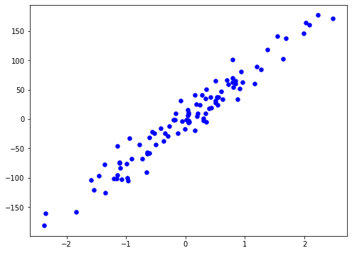
X, y = datasets.make_regression(n_samples=100, n_features=1, noise=20, random_state=5)
X_train, X_test, y_train, y_test = train_test_split(X, y, test_size=0.2, random_state=5)

fig = plt.figure(figsize=(8,6))
plt.scatter(X[:, 0], y, color="b", marker="o", s=30)
plt.show()

class LinearRegression:
    def __init__(self, lr=0.001, n_iters=1000):
        self.lr = lr
        self.n_iters = n_iters
        self.weights = None
        self.bias = None
        
    def fit(self, X, y):
        # init parameters 
        n_samples, n_features = X.shape
        self.weights = np.zeros(n_features)
        self.bias = 0
        
        # Gradient Descent 
        for _ in range(self.n_iters):
            # y = mx + c
            y_predicted = np.dot(X, self.weights) + self.bias
            # 2 in 2x can be ommited because it is a scaling factor
            dw = (1/n_samples) + np.dot(X.T, (y_predicted - y))
            db = (1/n_samples) + np.sum(y_predicted-y)
            
            # update parameters
            self.weights -= self.lr * dw
            self.bias -= self.lr * db
    
    def predict(self, X):
        y_predicted = np.dot(X, self.weights) + self.bias
        return y_predicted

def mse(y_true, y_predicted):
    return np.mean((y_true - y_predicted)**2)

regressor = LinearRegression(lr=0.01) #0.0001
regressor.fit(X_train, y_train)
predicted = regressor.predict(X_test)
mse_value = mse(y_test, predicted)
print("Linear Regression Mean Squared Error", mse_value)

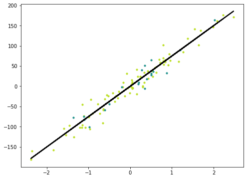
y_pred_line = regressor.predict(X)
cmap = plt.get_cmap('viridis')
fig = plt.figure(figsize=(8,6))
m1 = plt.scatter(X_train, y_train, color=cmap(0.9), s=10)
m2 = plt.scatter(X_test, y_test, color=cmap(0.5), s=10)
plt.plot(X, y_pred_line, color='black', linewidth=2, label='Prediction')
plt.show()

Linear Regression Mean Squared Error 305.7734835201333

Logistic Regression

Logistic Regression is used when the dependent variable(target) is categorical. Its a statistical analysis method to predict a binary outcome, such as yes or no, based on prior observations of a data set.

Approximation

Linear Function (countinuous values output)

f(w, b) = wx + b

Sigmoid Function (probabilistic output between 0-1)

s(x) = \frac{1}{1+e^{-x}}

\hat{y} = h_{0}(x) = \frac{1}{1+e^{-wx+b}}

Cost function

Cross entropy loss is reduced using gradient descent.

J(\hat{w}, b) = J(0) = \frac{1}{N}\sum^n_{i=1}[y^{i}log(h_{0}(x^{i}))+(1-y^{i})log(1-h_{0}(x^{i}))]

The main difference between linear and logistic regression is the sigmoid function applied to the output of a linear function

from sklearn import datasets
data = datasets.load_breast_cancer()
X, y = data.data, data.target
X_train, X_test, y_train, y_test = train_test_split(X, y, test_size=0.2, random_state=5)

class LogisticRegression:
    def __init__(self, lr=0.001, n_iters=1000):
        self.lr = lr
        self.n_iters = n_iters
        self.weights = None 
        self.bias = None
        
    def fit(self, X, y):
        # init parameters
        n_samples, n_features = X.shape
        self.weights = np.zeros(n_features)
        self.bias = 0
        for _ in range(self.n_iters):
            linear_model = np.dot(X, self.weights) + self.bias
            y_predicted = self._sigmoid(linear_model)
            
            # update weights  (2)
            dw = (1/n_samples) * np.dot(X.T, (y_predicted-y))
            db = (1/n_samples) * np.sum(y_predicted -y)
                
            self.weights -= self.lr * dw
            self.bias -= self.lr * db
        
    
    def predict(self, X):
        # using updated weights and bias
        linear_model = np.dot(X, self.weights)+self.bias
        y_predicted = self._sigmoid(linear_model)
        y_predicted_cls = [1 if i > 0.5 else 0 for i in y_predicted]
        return y_predicted_cls
        
    # helper method    
    def _sigmoid(self, x):
        return 1 / (1 + np.exp(-x))
        

def accuracy(y_true, y_pred):
    acc = np.sum( (y_true == y_pred)/ len(y_true))
    return acc

classifier = LogisticRegression(lr=0.0001) #0.0001
classifier.fit(X_train, y_train)
predicted = classifier.predict(X_test)
acc_value = accuracy(y_test, predicted)
print("Logistic Regression Accuracy ", acc_value)

Logistic Regression Accuracy  0.9298245614035088

Refactoring Regression Code

The linear and logistic regression code is similar apart from the sigmoid function transformation. We can create a base class that contains all the shared methods and properties.

class BaseRegression:
    def __init__(self, lr=0.001, n_iters=1000):
        self.lr = lr
        self.n_iters = n_iters
        self.weights = None
        self.bias = None
        
    def fit(self, X, y):
        n_samples, n_features = X.shape
        self.weights = np.zeros(n_features)
        self.bias = 0
        
        # Gradient Descent 
        for _ in range(self.n_iters):
            y_predicted = self._approximation(X, self.weights, self.bias)
            dw = (1/n_samples) + np.dot(X.T, (y_predicted - y))
            db = (1/n_samples) + np.sum(y_predicted-y)
            
            self.weights -= self.lr * dw
            self.bias -= self.lr * db
            
    # helper method to calculate the linear/sigmoid function value 
    def _approximation(self, X, w, b):
        raise NotImplementedError()
        
    # when predict method is called in base class output error
    def predict(self, X):
        return self._predict(X, self.weights, self.bias)
        
    def _predict(self, X, w, b):
        raise NotImplementedError()
    
class LinearRegressio(BaseRegression):
    def _approximation(self, X, w, b):
        return np.dot(X, w) + b
    
    def _predict(self, X, w, b):
        return np.dot(X, w) + b
    
class LogisticRegressio(BaseRegression):
    # _approximation returns probabilities like predict_proba
    def _approximation(self, X, w, b):
        linear_model = np.dot(X, w)+ b
        return self._sigmoid(linear_model)
    
    def _predict(self, X, w, b):
        linear_model =  np.dot(X, w) + b
        y_predicted = self._sigmoid(linear_model)
        #print(y_predicted[:90])
        y_predicted_cls = [1 if i > 0.5 else 0 for i in y_predicted]
        return y_predicted_cls
    
    def _sigmoid(self, x):
        return 1 / (1 + np.exp(-x))

clf = LogisticRegressio(lr=0.001) #0.0001
clf.fit(X_train, y_train)
predicted = clf.predict(X_test)

acc_value = accuracy(y_test, predicted)
print("Logistic Regresssion accuracy", acc_value)

Logistic Regresssion accuracy 0.9210526315789473

Support Vector Machines (SVM)

SVM algorithm is mostly used for classifiction problems, we plot each data item as a point in n-dimensional space with the value of each feature being the value of a particular coordinate. In classification we find the hyper-plane that best differentiates the classes.

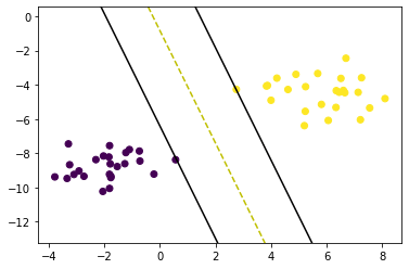
Uses a linear model to find a decision boundary(hyperplane) that best separates data classes. The margins between the hyperplane and the classes should be maximized (2 / ||w||).

Linear Model

w \cdot x - b = 0 \\ w \cdot x_i - b \ge 1 \ if \ y_i = 1 \\ w \cdot x_i - b \le -1 \ if \ y_i = -1 \\

y_i(w \cdot x_i - b) \ge 1

Cost Function

A cost function is a formula used to predict the cost that will be experienced at a certain activity level.

Hinge Loss

l = max(0, 1-y_i(w \cdot x_i - b))

l = \begin{cases} 0 & if \ \ y \cdot f(x) \ge 1 \\ 1 - y \cdot f(x) & otherwise. \end{cases}

Regularization

J = \lambda ||w||^2 + \frac{1}{n} \sum_{i=1}^n max(0, 1 - y_i(w \cdot x_i - b))

if \ \ y_i \cdot f(x) \ge 1: \ \ J_i = \lambda ||w||^2 \\ else: J_i = \lambda ||w||^2 + 1 - y_i(w \cdot x_i - b)

Gradients

if \ \ y_i \cdot f(x) \ge 1: \\ \frac{dJ_i}{dw_k} = 2\lambda w_k \\ \frac{dJ_i} {db} = 0 \\ else: \\ \frac{dJ_i}{dw_k} = 2\lambda w_k - y_i \cdot x_i \\ \frac{dJ_i}{db} = y_i

Update Rule

For each training sample $x_i$ :

w = w - \alpha \cdot dw \\ b = b - \alpha \cdot db

class SVM:
    def __init__(self, lr=0.001, lambda_param=0.01, n_iters=1000):
        self.lr = lr
        self.lambda_param = lambda_param
        self.n_iters = n_iters
        self.weight = None
        self.bias = None
        
    def fit(self, X, y):
        y_ = np.where(y <=0, -1, 1)  #convert [0,1] to [-1, 1]
        n_samples, n_features = X.shape
        
        self.weight = np.zeros(n_features)
        self.bias = 0
        
        for _ in range(self.n_iters):
            for idx, x_i in enumerate(X):
                condition = y_[idx] * (np.dot(x_i, self.weight) - self.bias) >= 1
                if condition:
                    self.weight -= self.lr  * (2 * self.lambda_param * self.weight)
                else:
                    self.weight -= self.lr * (2 * self.lambda_param*self.weight - np.dot(x_i, y_[idx]))
                    self.bias -= self.lr * y_[idx]
                    
    def predict(self, X):
        linear_output = np.dot(X, self.weight) - self.bias
        return np.sign(linear_output) # if positive: +1, if neg: -1
    
    
X, y = datasets.make_blobs(n_samples=50, n_features=2, centers=2, cluster_std=1.05, random_state=5)
X_train, X_test, y_train, y_test = train_test_split(X, y, test_size=0.2, random_state=5) 
y = np.where(y == 0, -1, 1)
clf = SVM()
clf.fit(X, y)

predictions = clf.predict(X)
acc = accuracy(y, predictions)

print("Svm Accuracy", acc)
print(clf.weight, clf.bias)



def visualize_svm():
    def get_hyperplane_value(x, w, b, offset):
        return (-w[0] * x + b + offset) / w[1]
    
    fig  = plt.figure()
    ax = fig.add_subplot(1, 1, 1)
    plt.scatter(X[:,0], X[:, 1], marker='o', c=y)
    
    x0_1  = np.amin(X[:, 0])
    x0_2 = np.amax(X[:, 0])
    
    x1_1 = get_hyperplane_value(x0_1, clf.weight, clf.bias, 0)
    x1_2 = get_hyperplane_value(x0_2, clf.weight, clf.bias, 0)
    
    x1_1_m = get_hyperplane_value(x0_1, clf.weight, clf.bias, -1)
    x1_2_m = get_hyperplane_value(x0_2, clf.weight, clf.bias, -1)
    
    x1_1_p = get_hyperplane_value(x0_1, clf.weight, clf.bias, 1)
    x1_2_p = get_hyperplane_value(x0_2, clf.weight, clf.bias, 1)
    
    ax.plot([x0_1, x0_2], [x1_1, x1_2], 'y--')
    ax.plot([x0_1, x0_2], [x1_1_m, x1_2_m], 'k')
    ax.plot([x0_1, x0_2], [x1_1_p, x1_2_p], 'k')
    
    x1_min = np.amin(X[:, 1])
    x1_max = np.amax(X[:, 1])
    ax.set_ylim([x1_min-3, x1_max+3])  # y-limits
visualize_svm()

Svm Accuracy 1.0
[0.58977016 0.17946483] -0.1520000000000001

KNN

The KNN algorithm is used for classification and regression problems. It assumes that similar things exist in close proximity to each other. We calculate distances between values using Euclidean distance.

$d = \sqrt{(x_2 - x_1)^2 + (y_2-y_1)^2)}$

from collections import Counter 

def euclidean_distance(x1, x2):
    # (sum(q_i-p_i)^2)^0.5
    return np.sqrt(np.sum( (x1-x2)**2))

class KNN:
    def __init__(self, k=3):
        self.k = k
        
    def fit(self, X, y):
        self.X_train = X
        self.y_train = y
    
    def predict(self, X):
        """
        Take each test item and pass it to _predict helper
        """
        predicted_labels = [self._predict(x) for x in X]
        return np.array(predicted_labels)
        
    def _predict(self, x):
        """
        Calculate the pythagorean distance between each test value and
        train items. 
        Select the k train rows with smallest distance.
        Find the most common class for the train rows with smallest distance
        
        """
        #compute distances
        distances = [euclidean_distance(x, x_train) for x_train in self.X_train]
        
        #get k nearest samples (shortest distance)
        k_indices = np.argsort(distances)[:self.k]
        k_nearest_labels = [self.y_train[i] for i in k_indices]
        #majority vote
        most_common = Counter(k_nearest_labels).most_common(1)
        return most_common[0][0] 

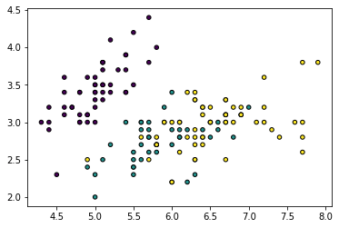
iris = datasets.load_iris()
X, y = iris.data, iris.target

X_train, X_test, y_train, y_test = train_test_split(X, y, test_size=0.2, random_state=1234)

plt.figure()
plt.scatter(X[:, 0], X[:, 1], c=y, cmap=cmap, edgecolor='k', s=20)
clf = KNN(k=2)
clf.fit(X_train, y_train)
predictions = clf.predict(X_test)
# sum of correct predictions / total test items
acc = np.sum( predictions == y_test)/len(y_test)
print("KNN accuracy", acc)   # k:5 = 0.97, k:3 = 1.0, k:2=1.0

KNN accuracy 1.0

Naive Bayes

Naïve Bayes is a probabilistic machine learning algorithm based on the Bayes Theorem, it is widely used in classification problems especially in natural language processing.

It assumes independence between predictors, in that the presence of a particular feature in a class is unrelated to the presence of any other feature.

Bayes Theorem

P(A|B) = \frac{P(B|A) \cdot P(A)}{P(B)} \\ P(y|X) = \frac{P(X|y) \cdot P(y)}{P(X)}

Assumption: All features are mutually independent

Probabilities: P(y|X)-posterior, P(x|y)-class conditional, P(y)- prior y, P(X) - prior x

P(y|X) = \frac{P(x_{1}|y) \cdot P(x_{2}|y) ... P(x_{n}|y)\cdot P(y)} {P(X)}

Select the class with the highest Probability

y = argmax_{y}P(y|X) = argmax_{y}\frac{P(x_1|y)\cdot P(x_2|y)\cdot P(y)} {P(X)} \\ y = argmax_y P(x_1|y)\cdot P(x_2|y)\cdot ... \cdot P(x_n|y).P(y) = argmax_y log(P(x_1|y))+log(P(x_2|y))+...+log(P(x_n|y))+log(P(y))

Log prevents overflow problems from very small numbers after multiplications Prior Probability P(y): frequency

Class conditional probability P(x_i|y): create probability density functions using normal distributions of different means and variances

P(x_i|y) = \frac{1}{\sqrt{2\pi \sigma_y^2}}\cdot exp(-\frac{(x_i - \mu_y)^2}{2\sigma_y^2})

class NaiveBayes:
    
    def fit(self, X, y):
        # each class means and variances
        n_samples, n_features = X.shape
        self._classes = np.unique(y)  #unique classes
        n_classes = len(self._classes)
        
        #init mean, var, priors
        self._mean = np.zeros((n_classes, n_features), dtype=np.float64)
        self._var = np.zeros((n_classes, n_features), dtype=np.float64)
        self._priors = np.zeros(n_classes, dtype=np.float64)
        
        for c in self._classes:
            X_c = X[c==y]             #filter rows with the class
            self._mean[c, :] = X_c.mean(axis=0)  #mean for rows
            self._var[c, :] = X_c.var(axis=0)
            self._priors[c] = X_c.shape[0] / float(n_samples) #class frequency
            
    def predict(self, X):
        y_pred = [self._predict(x) for x in X]
        return y_pred
        
    def _predict(self, x):
        posteriors = []
        for idx, c in enumerate(self._classes):
            prior = np.log(self._priors[idx])
            class_conditional = np.sum(np.log(self._pdf(idx, x)))
            posterior = prior + class_conditional
            posteriors.append(posterior)
        return self._classes[np.argmax(posteriors)]
            
    def _pdf(self, class_idx, x):
        # probility density function 
        mean = self._mean[class_idx]
        var = self._var[class_idx]
        numerator = np.exp(- (x-mean)**2 / (2*var))
        denominator = np.sqrt(2*np.pi*var)
        return numerator/denominator

X, y = datasets.make_classification(n_samples=100, n_features=10, n_classes=2, random_state=5)
X_train, X_test, y_train, y_test = train_test_split(X, y, test_size=0.2, random_state=5)

nb = NaiveBayes()
nb.fit(X_train, y_train)
predictions = nb.predict(X_test)

print("Naive Bayes Classifiction accuracy", accuracy(y_test, predictions))

Naive Bayes Classifiction accuracy 0.9500000000000002

Perceptron

A Perceptron is a linear machine learning algorithm for binary classification tasks. It is one of the simplest types of artificial neural networks, which is an important building block for deep learning.

A unit of a neural network, simulates the behavior of a cell. A cell receives an input signal and if it reaches a threshold it fires an output of 1 or 0.

Inputs > Weights > Net Input Function > Activation Function > Output

Linear Model

f(w, b) = w^Tx + b

Activation Function

Unit step function

g(z) = \begin{cases} 1 \ if \ z \ge 0 \\ 0 \ otherwise \end{cases}

Approximation

First apply the linear model function, then the activation function

\hat{y} = g(f(w,b)) = g(w^Tx+b)

Perceptron Update Rule

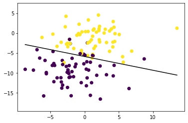
For each training sample, update new weight as old weight plus the delta weight. The delta weight is given by (alpha * (y-predictedy) * samplex). Alpha is the learning rate between [0,1].

w := w + \Delta w \\ \Delta w := a_i \cdot (y_i - \hat{y_i} \cdot x_i \\ \alpha : \ learning \ rate \ between \ [0,1]

In calculating the delta weight, if there is no difference between the actual and the predicted there is no change. However if there is a difference (misclassification) the weight increases(1-0=1) or decrease (0-1=-1)

Perceptron works for linearly seperable classes, to improve try different activation functions such as sigmoid function and in updating weights replace the perceptron update rule with gradient descent

class Perceptron:
    def __init__(self, lr=0.001, n_iters=1000):
        self.lr = lr
        self.n_iters = n_iters
        self.activation_func = self._unit_step_func
        self.weights = None
        self.bias = None 
    
    def _unit_step_func(self, x):
        return np.where (x >= 0, 1, 0)
    
    def fit(self, X, y):
        n_samples, n_features = X.shape
        
        # init weights 
        self.weights = np.zeros(n_features)
        self.bias = 0
        
        y_ = [1 if i > 0 else 0 for i in y]
        for _ in range(self.n_iters):
            for idx, x_i in enumerate(X):
                linear_output = np.dot(x_i, self.weights) + self.bias
                y_predicted = self.activation_func(linear_output)
                
                update = self.lr * (y_[idx] - y_predicted)
                self.weights += update * x_i
                self.bias += update 
        
    
    def predict(self, X):
        linear_output = np.dot(X, self.weights) + self.bias
        y_predicted  = self.activation_func(linear_output)
        return y_predicted 

X, y = datasets.make_blobs(n_samples=150, n_features=2, centers=2, cluster_std=3.05, random_state=5)
X_train, X_test, y_train, y_test = train_test_split(X, y, test_size=0.2, random_state=5)

p = Perceptron(lr=0.01, n_iters=1000)
p.fit(X_train, y_train)
predictions = p.predict(X_test)

print("Perceptron classification accuracy", accuracy(y_test, predictions))

fig = plt.figure()
ax = fig.add_subplot(1,1,1)
plt.scatter(X_train[:,0], X_train[:,1], marker='o', c=y_train)

x0_1 = np.amin(X_train[:, 0])
x0_2 = np.amax(X_train[:, 0])

x1_1 = (-p.weights[0] * x0_1 - p.bias) / p.weights[1]
x1_2 = (-p.weights[0] * x0_2 - p.bias) / p.weights[1]
ax.plot([x0_1, x0_2], [x1_1, x1_2], 'k')  # decision boundary

ymin = np.amin(X_train[:,1])
ymax = np.amax(X_train[:,1])
ax.set_ylim([ymin-3, ymax+3])

Perceptron classification accuracy 0.9666666666666667

Machine Learning From Scratch II (Continued)

To learn more about supervised methods e.g. Decision Trees, Random Forest, Linear Discriminant Analysis. Unsupervised methods e.g. K-Means, Principal Component Analysis

Linear Regression: Least Square Method

R Squared

Standard Error of the Estimate

Standard Deviation

Correlation

Implementing Linear Regression in Python

Cost Function

Gradient Descent

Update Rules

Logistic Regression

Approximation

Cost function

Refactoring Regression Code

Support Vector Machines (SVM)

Linear Model

Cost Function

Hinge Loss

Regularization

Gradients

Update Rule

KNN

Naive Bayes

Bayes Theorem

Select the class with the highest Probability

Perceptron

Linear Model

Activation Function

Approximation

Perceptron Update Rule

Machine Learning From Scratch II (Continued)

FURTHER READING