Decision Tree:

It has a tree-structure, where internal nodes represent the features of a dataset, branches represent the decision rules and each leaf node represents the outcome. It can be used for both regression and classification problems.

Entropy

Entropy is a measure of disorder or uncertainty and the goal of machine learning models is to reduce uncertainty. If the sample is completely homogeneous the entropy is zero and if the sample is an equally divided it has entropy of one

E = - \sum p(X) \cdot log_2(p(X)) \\ p(X) = \frac{x}{n}

Given S=[0,0,0,0,0,1,1,1,1,1]

E = -(\frac{5}{10}\cdot log_2(\frac{5}{10}) + \frac{5}{10}\cdot log_2(\frac{5}{10})) = 1

Information Gain

The information gain is the decrease in entropy after a dataset is split on an attribute. In the creation of a decision tree, we try to find an attribute that returns the highest information gain by having the most homogeneous branches.

IG = E(parent) - [weighted \ \ average] \cdot E(children)

Given S=[0,0,0,0,0,1,1,1,1,1], S1=[0,0,1,1,1,1,1], S2=[0,0,0]

IG = E(S) - [(7/10) * E(S1) + (3/10) * E(S2)] \\ IG = 1 - [(7/10) * 0.863 + (3/10) * 0] = 0.395

Training process

Starting at the top node, at each node select the best split based on the best information gain
Loop over all features and over all thresholds (greedy search all feature values)
Save the best split feature and split threshold at each node
Build the tree recursively
Apply some stopping criteria to stop growing e.g. maximum depth, minimum samples at node
When we have a leaf node, store the most common class label of this node

Prediction Process

Recursively traverse the tree
At each node look at the best split feature of the test feature vector x and go on the left or right depending on x[feature_idx] <= threshold
When we reach the leaf node we return the stored most common class label

from collections import Counter

def entropy(y):
    counts = np.bincount(y)  #count of occurences of class labels
    prob_y = counts/len(y)     # [3,6,9]/18 => 1/6, 1/3, 1/2
    return -np.sum([p*np.log2(p) for p in prob_y if p> 0])

class Node:
    def __init__(self, feature=None, threshold=None, left=None, right=None, *, value=None):
        self.feature = feature
        self.threshold = threshold
        self.left = left
        self.right = right
        self.value = value
        
    def is_leaf_node(self):
        return self.value is not None
    
class DecisionTree:
    def __init__(self, min_samples_split=2, max_depth=100, n_features=None):
        self.min_samples_split = min_samples_split
        self.max_depth = max_depth
        self.n_features = n_features
        self.root = None 
        
    def fit(self, X, y):
        # grow the tree
        self.n_features = X.shape[1] if not self.n_features else min(self.n_features, X.shape[1])
        self.root = self._grow_tree(X, y)
        
    def _grow_tree(self, X, y, depth=0):
        n_samples, n_features = X.shape
        n_labels = len(np.unique(y))
        
        #stopping criteria
        if (depth >= self.max_depth) \
            or n_labels == 1  \
            or (n_samples < self.min_samples_split):
            leaf_value = self._most_common_label(y)
            return Node(value=leaf_value)
        
        #randomly select a few features
        feat_idxs = np.random.choice(n_features, self.n_features, replace=False)
        # greedy search
        best_feat, best_thresh = self._best_criteria(X, y, feat_idxs)
        left_idxs, right_idxs = self._split(X[:, best_feat], best_thresh)
        # for each subset of rows find, best_criteria & split
        left = self._grow_tree(X[left_idxs, :], y[left_idxs], depth+1)
        right = self._grow_tree(X[right_idxs, :], y[right_idxs], depth+1)
        return Node(best_feat, best_thresh, left, right)
        
    def _best_criteria(self, X, y, feat_idxs):
        # find the feature and threshold with the highest info gain
        best_gain = -1
        split_idx, split_thresh = None, None
        for feat_idx in feat_idxs:
            X_column = X[:, feat_idx]
            thresholds = np.unique(X_column)
            for threshold in thresholds:
                gain = self._information_gain(y, X_column, threshold)
                
                if gain > best_gain:
                    best_gain = gain
                    split_idx = feat_idx
                    split_thresh = threshold
        return split_idx, split_thresh
    
    def _information_gain(self, y, X_column, split_thresh):
        # parent Entropy
        parent_entropy = entropy(y)
        
        # generate split
        left_idxs, right_idxs = self._split(X_column, split_thresh)
        
        if len(left_idxs) == 0 or len(right_idxs) == 0:
            return 0
        
        # weighted avearge child Entropy
        n = len(y)
        n_l, n_r = len(left_idxs), len(right_idxs)
        e_l, e_r = entropy(y[left_idxs]), entropy(y[right_idxs])
        child_entropy = (n_l/n) * e_l + (n_r/n) * e_r
        
        ig = parent_entropy - child_entropy
        return ig 
        
    def _split(self, X_column, split_thresh):
        left_idxs = np.argwhere(X_column <= split_thresh).flatten()
        right_idxs =np.argwhere(X_column > split_thresh).flatten()
        return left_idxs, right_idxs
    
    def _most_common_label(self, y):
        counter = Counter(y)
        most_common = counter.most_common(1)[0][0]
        return most_common 
        
    def predict(self, X):
        # traverse the tree
        return np.array([self._traverse_tree(x, self.root) for x in X])
    
    def _traverse_tree(self, x, node):
        if node.is_leaf_node():
            return node.value
        if x[node.feature] <= node.threshold:
            return self._traverse_tree(x, node.left)
        return self._traverse_tree(x, node.right)
        
data = datasets.load_breast_cancer()
X, y = data.data, data.target
X_train, X_test, y_train, y_test = train_test_split(X, y, test_size=0.2, random_state=5)

clf = DecisionTree(max_depth=10)
clf.fit(X_train, y_train)
y_pred = clf.predict(X_test)
acc = accuracy(y_test, y_pred)
print("Decision Tree accuracy:", acc
)

Decision Tree accuracy: 0.9210526315789473

Random Forest

Combines multiple trees each with a random subset of the data, predictions are made through majority voting by the trees. Multiple trees are better than a single tree in reducing overfitting and increasing accuracy

def bootstrap_sample(X, y):
    n_samples = X.shape[0]
    idxs =np.random.choice(n_samples, size=n_samples, replace=True)
    return X[idxs], y[idxs]

def most_common_label(y):
    counter = Counter(y)
    most_common = counter.most_common(1)[0][0]
    return most_common 

class RandomForest:
    def __init__(self, n_trees=100, min_samples_split=2, max_depth=100, n_features=None):
        self.n_trees =n_trees
        self.min_samples_split = min_samples_split
        self.max_depth = max_depth
        self.n_features = n_features
        self.trees = []
        
    def fit(self, X, y):
        self.trees = []
        for _ in range(self.n_trees):
            tree = DecisionTree(min_samples_split=self.min_samples_split, max_depth=self.max_depth, n_features=self.n_features)
            X_sample, y_sample = bootstrap_sample(X, y)
            tree.fit(X_sample, y_sample)
            self.trees.append(tree)
            
    def predict(self, X):
        tree_preds = np.array([tree.predict(X) for tree in self.trees])
        tree_preds = np.swapaxes(tree_preds, 0, 1) #convert rows to cols
        y_pred = [most_common_label(tree_pred) for tree_pred in tree_preds]
        return np.array(y_pred)
    
data = datasets.load_breast_cancer()
X, y = data.data, data.target
X_train, X_test, y_train, y_test = train_test_split(X, y, test_size=0.2, random_state=5)

clf = RandomForest(n_trees=5)  # try to optimize code for speed
clf.fit(X_train, y_train)
y_pred = clf.predict(X_test)
acc = accuracy(y_test, y_pred)
print("Random Forest accuracy:", acc)

Random Forest accuracy: 0.9298245614035088

AdaBoost

Boosting is an ensemble modelling technique that improves the prediction power by converting a number of weak learners to strong learners.

The idea behind boosting algorithms is to build a model on the training dataset, then a second model is built to reduce the errors in the first model. This procedure is repeated until the errors are minimized, and the predictions are correct.

Error

E_t = \frac{misclassifictions}{samples} = \frac{misclassifications}{n}

Misclassified is given a higher weight in the next iteration

E_t = \sum _{miss} weights

if error > 0.5, then error = 1- error

Weights

w_0 = \frac{1}{N} \ \ initial \ weight \ for \ each \ sample

Update rule to make sure there is more weight for misclassified samples

w = \frac{w \cdot exp(- \alpha \cdot y \cdot h(X)} { sum(w)}, \ \ where \ h(X) \ = \ prediction \ of \ t

Performance

\alpha = 0.5 \cdot log(\frac{1-E_t}{E_t})

Prediction

The sign of the sum of alpha times prediction. The better the learner the more it points to the positive or negative side.

y = sign(\sum_t^T \alpha _t \cdot h(X))

Training Process

Initialize weights for each sample = $\frac{1}{N}$ .

for t in T:

Train weak learner (find best feature and threshold)
Calculate the error for decision stump(1 feature tree split at a threshold) $E_t = \sum_{miss} weights$
- flip error and decision if error > 0.5
Calculate $\alpha = 0.5 \cdot log(\frac{1-E_t}{E_t})$
Update weights: $w = \frac{w \cdot exp(-\alpha \cdot h(X))}{Z}$

class DecisionStump:
    def __init__(self):
        self.polarity = 1  # +/- 1
        self.feature_idx = None
        self.threshold = None
        self.alpha = None
        
    def predict(self, X):
        n_samples = X.shape[0]
        X_column = X[:, self.feature_idx]
        
        predictions = np.ones(n_samples)
        if self.polarity == 1:
            predictions[X_column < self.threshold] =-1
        else:
            predictions[X_column > self.threshold] = -1
        return predictions

class Adaboost:
    def __init__(self, n_clf=5):
        self.n_clf = n_clf
        
    def fit(self, X, y):
        n_samples, n_features = X.shape
        
        # init weights
        w = np.full(n_samples, (1/n_samples)) #fill array of n with x
        
        self.clfs = []
        # greedy search all features & threshold
        for _ in range(self.n_clf): 
            clf = DecisionStump()
            min_error = float('inf')
            for feature_i in range(n_features):
                X_column = X[:, feature_i]
                thresholds = np.unique(X_column)
                for threshold in thresholds:
                    pol = 1
                    predictions = np.ones(n_samples)
                    predictions[X_column < threshold] = -1
                    
                    misclassified = w[y != predictions]
                    error = sum(misclassified)
                    
                    if error > 0.5:
                        error = 1- error
                        pol = -1
                    if error < min_error:
                        min_error = error
                        clf.polarity = pol
                        clf.threshold = threshold
                        clf.feature_idx = feature_i
        EPS = 1e-10  #prevent division by zero error              
        clf.alpha = 0.5 * np.log( (1-error) /(error+EPS))
        
        predictions = clf.predict(X)
        w *= np.exp(-clf.alpha * y * predictions) #exp(4) => 2.718**4
        w /= np.sum(w)
        
        self.clfs.append(clf)
        
    def predict(self, X):
        clf_preds = [clf.alpha * clf.predict(X) for clf in self.clfs]
        y_pred = np.sum(clf_preds, axis=0)
        y_pred = np.sign(y_pred)  #negatives/positives are -1/1
        return y_pred

data = datasets.load_breast_cancer()
X,y = data.data, data.target
y[y==0] = -1

X_train, X_test, y_train, y_test = train_test_split(X, y, test_size=0.2, random_state=5)

clf = Adaboost(n_clf=5)
clf.fit(X_train, y_train)
y_pred = clf.predict(X_test)
acc = accuracy(y_test, y_pred)
print("Adaboost accuracy: ", acc)

Adaboost accuracy:  0.9122807017543859

Unsupervised Machine Learning

It is a type of machine learning in which models are trained using unlabeled dataset. The goal of unsupervised learning is to find the underlying structure of dataset, group that data according to similarities, and represent that dataset in a compressed format.

Principal Component Analysis (PCA)

PCA finds a new set of dimensions such that all the dimensions are orthogonal (linearly independent) and are ranked according to their variance. The transformed features should be linearly independent, with the their dimensionality reduced as only the dimensions with the highest importance are kept. The new dimensions should minimize the projection error (near projection line) and the projected points should have the maximum spread/variance.

Variance

The deviation of the data from the mean:

Var(X) = \frac{1}{n} \sum (X_i - \hat{X})^2

Covariance Matrix

The level to which two variables vary together

Cov(X, Y) = \frac{1}{n} \sum(X_i - \hat{X})(Y_i - \hat{Y})^T

The autocovariance, is the covariation of a data point with another point of the same data.

Cov(X, X) = \frac{1}{n} \sum(X_i - \hat{X})(X_i - \hat{X})^T

Eigenvector & EigenValues

The eigenvector point in the direction of maximum variance, and the corresponding eigenvalues indicates the importance of its corresponding eigen vector.

A\hat v = \lambda \hat v \\ A \hat v = \lambda I v \\ Av - \lambda v = 0

When v is non-zero, we can solve the $\lambda$ using the determinant.

|A-\lambda I| = 0

A:matrix, v:eigenvector(direction that does not change) $\lambda$ : eigenvalue(scale of the stretch), I: Identity matrix

Given a matrix $\begin{bmatrix} -6 \ 3 \\ 4 \ 5 \end{bmatrix}$

|\begin{bmatrix} -6 & 3 \\ 4 & 5 \end{bmatrix} - \lambda \begin{bmatrix} 1 & 0 \\ 0 & 1 \end{bmatrix}| = 0 \\ \begin{vmatrix} -6 - \lambda & 3 \\ 4 & 5- \lambda \end{vmatrix} = 0

Calculating the determinant: (-6 - $\lambda$ )(5- $\lambda$ )- 3x4=0 => $\lambda ^2$ + $\lambda$ - 42 = 0 => $\lambda$ = -7 or 6

There are two possible eigenvalues $\lambda$ =-7 and $\lambda$ = 6. We can find their matching eigenvectors as follows.

\begin{bmatrix} -6 & 3 \\ 4 & 5 \end{bmatrix} \begin{bmatrix} x \\ y \end{bmatrix} = 6 \begin{bmatrix} x \\ y \end{bmatrix}

After multiplying we get two equations:

-6x + 3y = 6x \\ 4x + 5y = 6y

Bring all to the left:

-12x + 3y = 0 \\ 4x - 1y = 0 \\ 4x = y

For eigenvalue $\lambda$ =6, the eigenvector is any non-zero multiple of $\begin{bmatrix} 1 \\ 4 \end{bmatrix}$

Av = \lambda v \\ \begin{bmatrix} -6 & 3 \\ 4 & 5 \end{bmatrix}\begin{bmatrix} 1 \\ 4 \end{bmatrix} = \begin{bmatrix} -6*1+3*4 \\ 4*1+5*4 \end{bmatrix} = \begin{bmatrix} 6 \\ 24 \end{bmatrix} = 6 \begin{bmatrix} 1 \\ 4 \end{bmatrix}

PCA process

Subtract the mean from X
Calculate Cov(X, X)
Calculate eigenvectors and eigenvalues of covarance matrix
Sort the eigenvectors according to the eigenvalues in decreasing order
Choose the first k eigenvectors and that will be the new k dimensions
Transform the original n dimensional data points into k dimesions(Projection with dot product)

class PCA:
    def __init__(self, n_components):
        self.n_components = n_components
        self.components = None
        self.mean = None
        
    def fit(self, X):
        # mean 
        self.mean = np.mean(X, axis=0) #mean per row
        X = X - self.mean
        #covariance
        cov = np.cov(X.T)  #column covariance
        
        #eigen vectors & eigenvalues
        eigenvalues, eigenvectors = np.linalg.eig(cov)
        
        #sort eigenvectors
        eigenvectors = eigenvectors.T   # returned as one column
        idxs = np.argsort(eigenvalues)[::-1] #reverse a list
        eigenvalues = eigenvalues[idxs]
        eigenvectors = eigenvectors[idxs]
        #store first n eigenvectors (n_components by X.shape[1])
        self.components = eigenvectors[0:self.n_components]
        
        
    def transform(self, X):
        # project data
        X = X - self.mean
        return np.dot(X, self.components.T)  #convert to columns
        
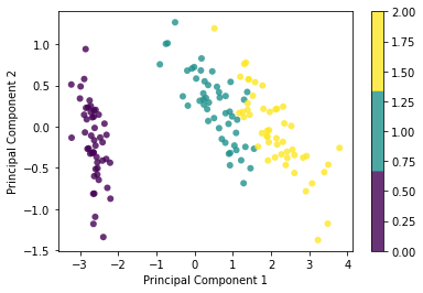
data = datasets.load_iris()
X = data.data
y = data.target

pca = PCA(2)
pca.fit(X)
X_projected = pca.transform(X)

print("Shape of X: ", X.shape)
print("Shape of transformed X:", X_projected.shape)

x1 = X_projected[:, 0]
x2 = X_projected[:, 1]
plt.scatter(x1, x2, c=y, edgecolor='none', alpha=0.8, cmap=plt.cm.get_cmap('viridis', 3))
plt.xlabel('Principal Component 1')
plt.ylabel('Principal Component 2')
plt.colorbar()
plt.show()

Shape of X:  (150, 4)
Shape of transformed X: (150, 2)

Linear Discriminant Analysis

LDA is a feature reduction technique that projects a dataset onto a lower-dimensionality space with good class-separability by maximizing the component axes for class-separation.

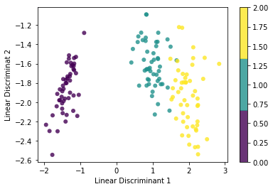
PCA is unsupervised and finds the component axes that maximizes the data variance, LDA is a supervised method that finds axes that maximize the separation between classes.

Within class scatter matrix

S_W = \sum _c S_c \\ S_c = \sum _{i \in c} (x_i - \vec{x}_c) \cdot (x_i - \vec{x}_c)^T

Between class scatter matrix

S_B = \sum _c n_c \cdot (\vec{x}_c - \vec{x}) \cdot (\vec{x}_c - \vec{x})^T

Eigenvalue & Eigenvector

S_W^{-1} S_B

LDA Process

Calculate $S_B \ and \ S_W$
Calculate eigenvalues of $S_W^{-1}S_B$
Sort the eigenvectors according to their eigenvalues in decreasing order
Choose first k eigenvectors as the new k dimensions
Transform the original n dimensional data points into k dimensional by projection with dot product

class LDA:
    def __init__(self, n_components):
        self.n_components = n_components
        self.linear_discriminants = None  #store eigenvectors
        
    def fit(self, X, y):
        n_features = X.shape[1]
        class_labels = np.unique(y)
        
        #S_W & S_B
        mean_overall = np.mean(X, axis=0)
        S_W = np.zeros((n_features, n_features))
        S_B = np.zeros((n_features, n_features))
        
        for c in class_labels:
            X_c = X[y == c]
            mean_c = np.mean(X_c, axis=0)
            S_W += (X_c - mean_c).T.dot(X_c - mean_c)
            
            # Between class
            n_c = X_c.shape[0]
            mean_diff = (mean_c - mean_overall).reshape(n_features, 1) #rows * col
            S_B  += n_c * (mean_diff).dot(mean_diff.T)
        A = np.linalg.inv(S_W).dot(S_B)  #matrix
        eigenvalues, eigenvectors = np.linalg.eig(A)
        eigenvectors = eigenvectors.T
        idxs = np.argsort(abs(eigenvalues))[::-1]
        eigenvalues = eigenvalues[idxs]
        eigenvectors = eigenvectors[idxs]
        self.linear_discriminants = eigenvectors[0:self.n_components]
        
        
    def transform(self, X):
        return np.dot(X, self.linear_discriminants.T)
    
data = datasets.load_iris()
X, y = data.data, data.target

# Project the data onto the 2 primary linear discriminants
lda = LDA(2)
lda.fit(X, y)
X_projected = lda.transform(X)
print('Shape of X:', X.shape)
print('Shape of transformed X:', X_projected.shape)

x1 = X_projected[:, 0]
x2 = X_projected[:, 1]
plt.scatter(x1, x2, c=y, edgecolor='none', alpha=0.8, cmap=plt.cm.get_cmap('viridis', 3))
plt.xlabel('Linear Discriminant 1')
plt.ylabel("Linear Discriminat 2")
plt.colorbar()
plt.show()

KMEANS

An unsupervised machine learning method that clusters a dataset into k different clusters. Each sample is assigned to the cluster with the nearest mean.

Iterative optimization

Initialize clusters centers randomly
Assign points to the nearest cluster center (centroid)
Repeat until convergence to update cluster labels
Set the center to the mean of each cluster
Repeat until convergence to update cluster centroids

Euclidean distance

Get the distance between two feature vectors

d(p, q) = \sqrt { \sum (p_i - q_i)^2 }

from sklearn.datasets import make_blobs

np.random.seed(42)
import matplotlib.pyplot as plt

def ecudlidean_distance(x1, x2):
    return np.sqrt(np.sum((x1-x2)**2))

class KMeans:
    def __init__(self, K=5, max_iters=100, plot_steps=False):
        self.K = K
        self.max_iters = max_iters
        self.plot_steps = plot_steps
        # list of sample indices for each cluster
        self.clusters = [[] for _ in range(self.K)]
        # mean feature vector for each cluster
        self.centroids = []
    
    def predict(self, X):
        self.X = X
        self.n_samples, self.n_features = X.shape
        
        # init centroids 
        random_sample_idxs = np.random.choice(self.n_samples, self.K,  replace=False)
        self.centroids = [self.X[idx] for idx in random_sample_idxs]
        
        # optimization
        for _ in range(self.max_iters):
            # update clusters
            self.clusters = self._create_clusters(self.centroids)
            if self.plot_steps:
                self.plot()
            # update centroids 
            centroids_old = self.centroids
            self.centroids = self._get_centroids(self.clusters)
            if self.plot_steps:
                self.plot()
            # check if converged 
            if self._is_converged(centroids_old, self.centroids):
                break    
        # return cluster labels 
        return self._get_cluster_labels(self.clusters)
    
    def _get_cluster_labels(self, clusters):
        labels = np.empty(self.n_samples)  #empty creates array of set shape
        for cluster_idx, cluster in enumerate(clusters):
            for sample_idx in cluster:
                labels[sample_idx] = cluster_idx
        return labels
        
    def _create_clusters(self, centroids):
        clusters = [[] for _ in range(self.K)]
        for idx, sample in enumerate(self.X):
            centroid_idx = self._closest_centroid(sample, centroids)
            clusters[centroid_idx].append(idx)
        return clusters
    
    def _closest_centroid(self, sample, centroids):
        distances = [ euclidean_distance(sample, point) for point in centroids]
        closest_idx = np.argmin(distances)
        return closest_idx
    
    def _get_centroids(self, clusters):
        centroids = np.zeros((self.K, self.n_features))
        for cluster_idx, cluster in enumerate(clusters):
            cluster_mean = np.mean(self.X[cluster], axis=0)
            centroids[cluster_idx] = cluster_mean
        return centroids
    
    def _is_converged(self, centroids_old, centroids):
        distances = [euclidean_distance(centroids_old[i], centroids[i]) for i in range(self.K)]
        return sum(distances) == 0
    
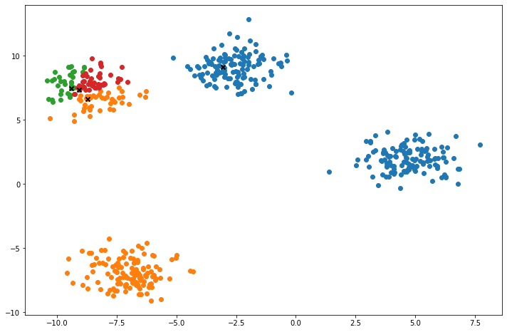
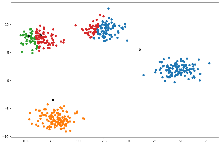
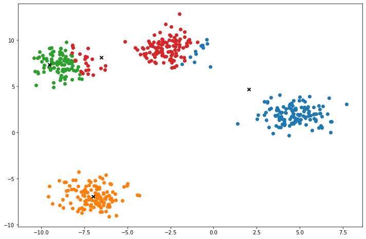
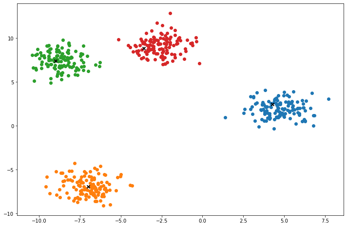
    def plot(self):
        fig, ax = plt.subplots(figsize=(12, 8))
        for i, index in enumerate(self.clusters):
            point = self.X[index].T
            ax.scatter(*point)
        for point in self.centroids:
            ax.scatter(*point, marker='x', color='black', linewidth=2)
        plt.show()
        
X, y = make_blobs(centers=4, n_samples=500, n_features=2, shuffle=True, random_state=5)
clusters = len(np.unique(y))
print("clusters:", clusters)

k = KMeans(K=clusters, max_iters=150, plot_steps=True)
y_pred = k.predict(X)

Cluster 4

Machine Learning in practice

Machine learning is applied in pattern and image recognition, web search results, fraud detection, credit scoring, and in serving adverts on webpages. In conclusion, machine learning can produce accurate results and analysis from big data by developing fast and efficient algorithms for real-time data processing.

Machine Learning From Scratch II