In Statistic and Probability Overview I, we covered hypothesis testing, confidence intervals, parametric tests, non-parametric tests, p-values, effect-size and inferential statistics by bootstrapping. In this piece, we explore regression analysis, timeseries analysis, Monte Carlo Simulations and Markov Chains.

Regression Analysis

It is an inferential method that models the relationship between a dependent/response variable and one or more predictor variables. The goal is to draw a random sample from a population and to use it to produce coefficients that estimates properties of the population.

A regression model has a constant and a coefficient multiplied by an independent variable. The constant absorbs the bias emanating from residuals(errors) that have a positive or negative mean.

$Y = \beta_0 + \beta_1X_1 + ...+ \beta_kX_k + \epsilon$

Linear regression is also called ordinary least square (OLS) is prone to overfitting due to presence of outliers and multicollinearity.

Advanced regression methods

Ridge: used with data with severe multicollinearity. Reduce variance caused by multicollinearity by introducing a slight bias in estimates
Lasso: Similar to Ridge but selects variables thereby creating a simpler model
Partial Least Squares (PLS): used with few observations/multicollinearity. It works by performing feature reduction like PCA to create fewer uncorrelated components.
Nonlinear regression
Poisson: how change in independent variables is associated with count of events over a time period. When data variance is not equal to the mean, use replace poisson with negative binomial regression. When the output has too many zeros, replace poisson with zero-inflated models.

Regression assumptions (error/residual=observed-predicted)

The linear model residuals have a mean of zero, have no correlation with themselves and other variables and have a constant variance.

the model is linear with (coefficients*independent + error)
the error is random/stochastic with an average of zero, we use a constant to offset error/bias.
independent variables are uncorrelated with the error, not a single independent variable has influence on error
errors are uncorrelated. If the errors are positive or negative correlated(autocorrelation) like in time series data. To remove cyclical/trending residuals, use an independent variable that captures the information or distributed lag models
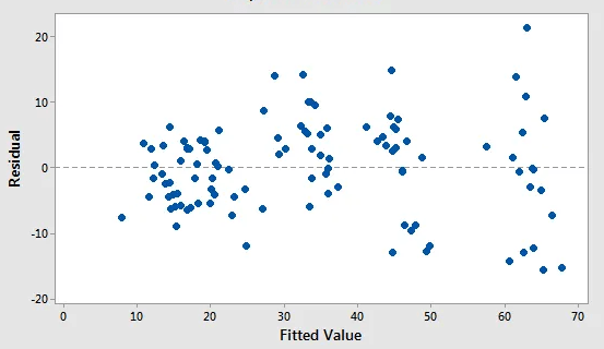
the errors have a constant variance(homoscedasticity). There is no cone shape when we scatter residuals vs predicted/fitted

No independent/explanatory variable is highly correlated with another, multicollinearity
the errors are normally distributed, can be used to generate reliable confidence intervals

Avoid making a prediction for a point that is outside the range of observed values that were used to fit the regression model as the relationship can change outside

Logistic Regression

Describes relationship between a set of independent variables and a categorical dependent variable

Types of Logistic regression

Binary: two possible values in the dependent variable
Ordinal: has at least 3 ordinal responses e.g. hot, medium, cold
Nominal/multinormal: has at least 3 groups that do not have natural order e.g. red, white, blue

Independent variables: predictors, features, factors, treatment variables, explanatory, inputs, X-variables and right-hand variables

Nonlinear Regression (independent vs predicted forms a curve)

To detect nonlinear relationship plot each independent vs predicted/fitted, check if the line is straight or curved. Use the predicted vs residual to check for regression assumptions eg error is random. For nonlinear, the R-squared is inaccurate and p-values are invalid, we have to focus on reducing the standard error i.e. as compared to a linear model.

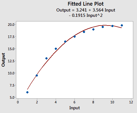
Curve fitting is the process of specifying the model that provides the best fit to the specific curves in the data. The most common method is to include polynomial terms in the linear model e.g. $x^2, x^3$ . To determine the correct polynomial, count the number of bends in the line and add one e.g. quadratic ( $x^2$ ) for one bend, cubic ( $x^3$ ) for two bends.

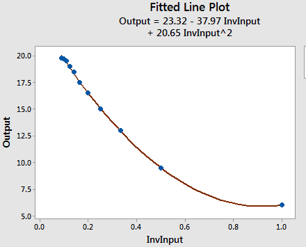
We use reciprocal $\frac{\beta * 1}{X}$ terms in linear regression, when the dependent variable descends to the floor or ascends to the ceiling.

Another approach is log transformations in double form(boths sides) e.g. $Y= e^{BO}X_1^{B1}X_2^{B2} \rightarrow ln Y = B_0 + B_1lnX_1 + B_2lnX_2$ or semi-log e.g. $output = 6.2 + 14.5 log(inputX)$

The best metric for evaluating curve fitted models is standard error. We combine curve fitting approaches to find the best fit for the dataset e.g. reciprocal-quadratic model.

Interpreting Results of a Regression Analysis

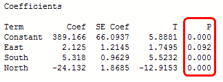
The p-value determines whether what is seen in the sample exists in the population. If it is less than the significance level, the sample provides enough evidence to reject the null hypothesis that states that a variable has no correlation with the dependent variable.

The p-values determines what variables to include in the final model, in this case include all except East which is statistically insignificant. Having a positive coefficient indicates that as the independent variable increases the mean of the dependent variable increase. The coefficient value is how much the mean of the dependent varible changes given a one-unit change in the independent variable while holding other variables constant. A unit increase in East will cause 2.125 in the dependent variable.

By scattering an independent vs dependent variable, the slope of the regression line can be positive, negative or zero. If zero, the coefficient is zero and there is no correlation. If the slope is positive, the correlation is positive.

R-Squared ( $R^2$ )

It is a goodness of fit measure that indicates the percentage variance in the dependent variable that can be explained by independent variables.

R^2 = \frac {Explained Variance}{Total Variance}

Residual plots can find a biased model that has a high $R^2$ . A good model has unbiased differences between the observations and the predicted values. Unbiased predictions are not too high or too low at any point of the curve.

Polynomial variables

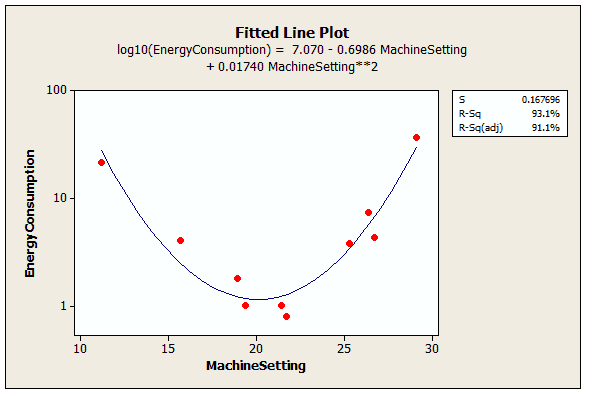
The chart shows how the effect of machine setting on mean energy consumption depends on where you are on the regression curve. Moving away on both sides from machine setting at 20 leads to increase in energy consumption.

Interaction Effects

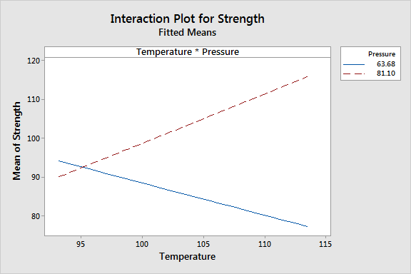
Interaction effects occur when the effect of one variable depends on the value of another variable. Statistically significant interaction effects must be considered together with the main(single variable) effects. The temperature effect on strength depends on whether the pressure is low or high. For low pressure increase in temperature reduces strength,and for high pressure increase in temperature increases strength.

Regression coefficients are unstandardized as they retain the natural units of the dependent variable

Omitted/Confounding/lurking variables

Important variables not included in the model and therefore cannot be controlled leading to distorting the effect due ommited variable bias. A confounding variable must correlate with the dependent variable and with at least one of the independent variables. If the confounding variable is not correlated with an independent variable then it does not produce bias, and if it has a weak correlation with the dependent variable then the bias is small. Omitted variable bias occurs in observational studies, random sampling in experiments reduces the effect of confounding variables (as effect is distributed across all groups).

A thorough literature review helps to avoid omitting an important variable, we can also use a proxy variable that is highly correlated with an ommitted variable that is hard to collect data.

In Observational studies we do not interfere with the subject of the study, we have explanatory variables and response variables that have correlation relationships. However, randomized experimental studies have independent/controlled and dependent variables with causal relationships. An observation study could be survey data on strikers asking the amount of hours spent on training and the number of goals scored. Whereas, a randomized experiment could be treatment and control(placebo) groups testing the effects of a vaccine.

Time Series Analysis

Time series analysis tracks the characteristics of a process at regular time intervals to understand how a metric changes over time. They are a set of measures that occur at regular time intervals. Time series analysis seeks to understand patterns in changes over time such as trends, cycles and irregular movements. Applied in monthly sales, prices, birth & death rates, stock & GDP, climate change

Time series is a sub-type of panel data which tracks multiple characteristics, time series only tracks a single characteristic i.e. time variable and characteristic variable. Time series data is longitudinal that looks at many points in time, Cross-sectional data is collected at a single point in time to determine differences between subjects. Time series has an element of direction in the sense that past events influence the future and not vice-versa, and events closer together have stronger association than more distant observations.

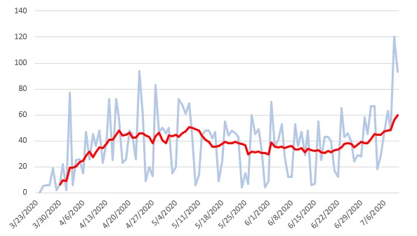
Random fluctuations can obscure the underlying patterns, smoothing techniques cancel out fluctuations to reveal trends and cycles.

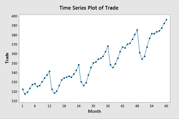
A time series has cycles of patterns mostly of fixed length that repeat with or without a longterm trend.

Smoothing Timeseries Data with Moving Averages

Smoothing or filtering is the process of removing random variations in time series data to reduce noise and amplify cycles and trends. Moving average is based on the belief that observations that are close in time are likely similar. Moving averages are a series of averages calculated using sequential segments of data points over a series of values. Their length is number of data points to include in each average

One-sided moving average

It includes the current and the previous observations for each average. The MA of at a time t with length of 3 is given by;

MA_3 = \frac{X_{t-2} + X_{t-1} + X_t}{3}

Centered moving average

It includes previous and future observations, uses observations that surround it in both directions/two-sided.

MA_5 = \frac{X_{t-2} + X_{t-1} + X_{t} + X_{t+1} + X_{t+2}}{5} \\ MA_6(even) = \frac{(0.5*X_{t-3}) + X_{t-2} + X_{t-1} + X_{t} + X_{t+1} + X_{t+2} + (0.5*X_{t+3})}{6}

For a seasonal pattern in the data, choose a length of MA equal to pattern's length to remove the seasonality and to show the underlying trends. For data affected by low activity over the weekend, use a 7-day MA length. Longer lengths produce smoother lines.

Exponential Smoothing for Time Series Forecasting

Produces forescasts that are weighted averages of past observations with the weights of older observations exponentially decreasing. It models Error, Trend and Seasonality (ETS) by adjusting parameters to relative importance of new to older observations as required. Moving Averages give equal weights to all observations in the window and zero weight to observations outside the window.

Simple/Single Exponential Smoothing (SES)

It estimates the level component(typical value/average) using an alpha value between 0 to 1. Lower values give more weight to past observations by averaging fluctuations over time to produce smooth lines. A high alpha ( $\alpha$ ) allows forecast to have quick reaction to changing conditions but makes it more sensitive to noise(fluctuations). SES forecasts are equal to the last level component making it only appropriate for data without trend or seasonality. A popular metric for prediction accuracy in forecasting is Mean Absolute Percentage Error (MAPE)

MAPE = \frac{1}{n} \sum_{t=1}^n | \frac{A_t - F_t}{A_t}|

n: number of times summation iteration happens, A: actual, F: forecast

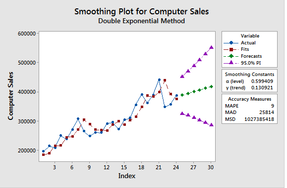
Double Exponential Smoothing (DES) or Holt's Method

Adds support for trends by adding a decay factor Beta $(\beta)$ . To prevent the trend from continuing into unrealistic values, add a damping coefficient Phi ( $\phi$ ). A trend can be additive with a constant scale as observations change or multiplicative that magnitude increase with data increase.

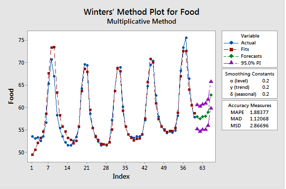
Triple Exponential Smooting (TES)

Add the support for seasonality by adding a gamma $(\gamma)$ parameter.

Time Series Data AutoCorrelation and Partial Autocorrelation

Autocorrelation Function (ACF) is correlation between two observations at different points/intervals in a time series that shows past values influence on recent value. Lags are the number of intervals between two observations, previous has a lag=1, interval before that has lag=2.

AutoCorrelation Function (ACF) = $Corr(y_t, y_{t-k}), k=1,2...$ | k is lag

For random data, autocorrelation for all lags is zero (whitenoise).

Stationarity: without seasonality or trend, and the variance and autocorrelation is constant. Stationarity data autocorrelation declines rapidly to zero.

Trends: short lags for data with trend has large positive correlation because observations closer in time tend to have similar values

Seasonality: lags at multiples of seasonal frequency have larger autocorrelation

Partial Autocorrelation Function (PACF)

PACF function is similar to ACF, except it displays only the correlation between two observations that the shorter lags between those observations do not explain. For lag 3, display correlation that lags 1 and 2 do not explain. The goal is to only describe the direct relationship between an observation and its lag by removing the indirect correlations caused by linear function of correlation of the observation with observations at the intervening time steps.

Auto Regressive means a linear regression model uses its own lags as predictors. ACF determines whether auto-regressive model is needed, then PACF help choose the model terms.

ARIMA(p,d,q) Models

Auto Regressive Moving Integrated Moving Average (ARIMA) is a forecasting algorithm that uses its own lags and lagged forecast errors of past time series values to predict future values. The prediction process involves

Auto Regression: linear regression model that uses own lags(p) as predictors
Stationarity: uses differencing(d) by subtracting previous value from the current value
Moving Average: number of lagged forecast errors(q) to include

Predicted(Yt) = Constant + Linear combination Lags of Y(p) + Linear Combination of Lagged forecast errors(q)

Y_t = \alpha + \beta_1 Y_{t-1} + \beta_2 Y_{t-2} + .. + \beta_pY_{t-p} \epsilon_{t} + \phi_1 \epsilon_{t-1} + \phi_2 \epsilon_{t-2}+..+\phi_q \epsilon_{t-q}

Monte Carlo Simulations

This a computerized mathematical technique that enable accounting for risk in quantitative analysis and decision making.

4 Steps in conducting a Monte Carlo simulation

Identifying the transfer equation: the business formula
Define the input parameters: the probability distribution of inputs
Set up the simulation: creating a very large random data such as 10^6 instances
Use the business formula to calculate the simulated outcomes

Monte Carlo Simulation Exampe 1

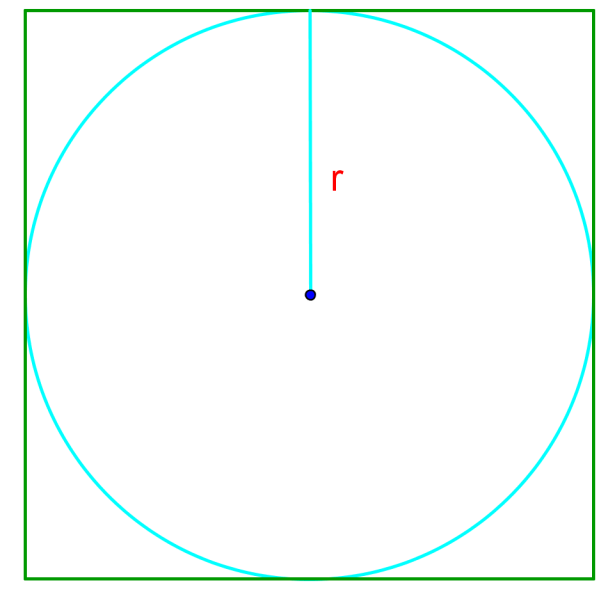
Given a square of 2x2 units, that has a circle inside that touch all sides. What is the probability that if you select a point inside the square, it will be inside the circle.

Solving the problem by mathematical analysis

rectagle_area: L * W => 2 * 2 = 4
circle_area: Diameter=2, radius=1, $\pi r^2$ = $\pi * 1^2 = \pi$
P(Circle) = $\frac{desired}{totalOutcomes}$ = $\frac{\pi}{4} =0.7857$

"""
For any value inside a circle (x**2 + y**2 <= radius**2). 
The x and y values bigger than the radius squared are deemed to be outside the circle. 
   rectangle: x: -1, 1, and y: -1, 1  |x|=2, |y|=2
   circle: diameter=2, radius=1
"""
import numpy as np
import random 

n=100000
inside = 0

for i in range(n):
    x = random.uniform(-1,1)  
    y = random.uniform(-1, 1)
    area = (x**2) + (y**2)
    if area <= 1:
        inside += 1

print("The Probability of landing inside the circle is": inside/n)

The Probability of landing inside the circle is 0.7868

Monte Carlo Simulation Example 2

Given a game where P(win) = p, the game ends if you lose 2 rounds in a row. What is the expected number of rounds we are going to play when;

the probability of winning is 75%?
the probability of winning is 45%?

Solution by mathematical analysis

$Expected\ rounds\ (p=0.75) = \frac{2-p}{(1-p)^2} = \frac{2-0.75}{(1-0.75)^2} = 20$
$Expected\ rounds\ (p=0.45) = \frac{2-p}{(1-p)^2} = \frac{2-0.45}{(1-0.45)^2} = 5.1240$

Solution by Monte Carlo Simulation

p = 75;      #p=45
rounds= []
for _ in range(n):
    play=True
    loss = 0
    count = 0
    while play:
        count += 1
        
        x = random.choice(np.linspace(1, 100, 100))
        if x > p :
            loss += 1
        else :
            loss = 0
            
        if (loss >= 2):
            play = False
    rounds.append(count)   
print(f"Number of rounds when p={p/100} is {sum(rounds)/n}")

Number of rounds when p=0.75 is 19.99273
Number of rounds when p=0.45 is 5.11602

The time taken in monte carlo simulations can increae exponentially as the n gets larger thereby slowing down the process

Markov Chains

A Markov chain is a mathematical system that experience transistion from one state to another according to certain probabilistic rules. It models a sequence of possible events in which the probability of each event depends only on the current state. The states exist at a certain point in time and can change depending on the transition matrix.

Example of application of Markov Chains

In a market dominated by two companies, at present Company A has 55% of market share, Company B has 45%. The probability of a B customer staying over the next one year is 70% as 30% switch to A, and the probability of an A customer switching to B is 10% as 90% remain. What is the future market share for each company after 1 yr.

\begin{bmatrix} Current\ State \\ A & B \\ 0.55 & 0.45 \end{bmatrix} X \begin{bmatrix} Transition\ Matrix \\ 0.7 & 0.3 \\ 0.1 & 0.9 \end{bmatrix} = \begin{bmatrix} Final\ State \\ A & B \\ 0.43 & 0.57 \end{bmatrix}

Future Market share for Company A = (0.55x0.7) + (0.45x0.1) = 43%

Statistics and Probability Overview III (Continued)

To learn more about Probability, Permutations and Combinations, Probability Distributions, and Data Visualization