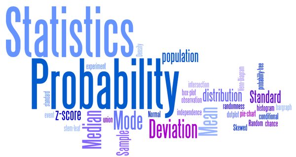
Statistics and Probability Overview I

Statistics is the study and manipulation of data, including ways to gather, review, analyze, and draw conclusions for better decision making. It is the science of learning from data.

In statistics we study populations and samples. A population is the set of all similar items that exists. Populations parameters are mostly unknowable such as mean( $\mu$ ) and the standard deviation( $\sigma$ ). A sample is a subset of a population. Sample statistics such as mean, and standard deviation are estimates. The sampling error is the difference between the sample statistic and the population parameter.

Variability/spread of each observation from the mean is the Standard Deviation, Standard Error of the Mean is the variability of sample means in a sampling distribution of means. Standard Error is caused by sampling error, it indicates how far(precision) the sample mean is from the population mean using the original measurement units.

$SEM = \frac{\sigma}{\sqrt{N}}$

The larger the sample size, the smaller the standard error which results in smaller p-values and confidence intervals, which is desirable.

There are two major methods of statistics:

Descriptive: used to summarize(5 numbers: min,max,Q1,median,Q3) and graph data
- Central tendency measures of a population or sample like mean,mode, & median.
- Dispersion which ist the difference between members of a sample using variability measures like range, variance/spread & standard deviation
- Skewness which is the shape of the data as visualized by a dot-plot(few values) or histogram. Also, the kurtosis and probability distribution(discrete)/density(continuous) function
Inferential: takes a sample and make inferences about the larger population.
- Sampling results are estimates/uncertain and are affected by sampling error. The results are presented as a point estimate (mean), standard deviation, and confidence intervals.
- Random sampling aims at finding a sample that mirrors the population. In finding a representative sample we use simple random sampling, systemic sampling, stratified sampling & cluster sampling
- Non-probability/random sampling methods are good for piloting a study or survey instruments but their results cannot be generalized to the general population. Sampling subjects by availability in convinience sampling is easy eg on social media. Other non-random methods include snowball (drug addicts), quota (female/male), purposive (experts)
- Popular methods in inferential statistics are hypothesis testing, confidence intervals and regression analysis.

Law of large numbers states that as sample size grows, the sample statistics (mean) will converge on the population value

5 Steps for Conducting Scientific Studies with Statistical Analyses

The scientific method requires experimentation and statistical analysis. The process has to be rigorous and thorough to obtain valid results.

Research Phase
- Define the problem and the research question that is clear and concise.
- what has been done, whether a new study or replicating a study
- Literature review to gain in-depth knowledge about the subject matter
- give current state of scientific knowledge on the research question
- how previous research was done; variables, measurements, sampling, design, analysis
Operationalization Phase
- Define the right variables & measurement techniques that are precise & accurate.
  - Find the location, best sampling method & sample size i.e. power analysis
- Design the experimental methods whether observational or experimental
  - compare means or proportions or relationships
  - one vs two-tailed tests
  - Limit the number of tests as the more the test the higher the error rate
  - bonferroni correction: for n independent hypothesis, signficance level is 0.05/n.
Data collection; the instruments to use e.g. surveys questionaires, lab
Statistical analysis and conclusion; validate data, test assumptions, analyse
Communicate the results; hypothesis favored, share enough details for replication

Some major pitfalls in statistical studies;

Biased samples: incorrectly sample the subjects
Inaccuracies and lack of precision in the data collection methods
Overgeneralization: apply findings to a different population
Causality: mistaking correlation for causality ie without conducting a random assignment experiment
Incorrect analysis: applying a linear model to non-linear variables, wrong statistical test or use mean where median would be a better option
P-hacking: when a test is repeated many times, statistically significant results can be due to chance

A sample statistic estimates a population parameter, a point estimator can be biased(not equal), unbiased (equal) or asymptotically unbiased when the estimator approaches the population value as the sample size increases.

Reliability vs Validity in Research

Reliability is the consistency of the measure with same results under the same conditions across time. Validility is whether measurements reflect what they are supposed to measure or they reflect something else. Valid measures are consistent with the theory, and other similar measures.

Assessing reliability (consistency)

test and later retest
internal reliability (high correlation with other measures for the same characteristic).
inter-rater reliability by using different observers or evaluators

Assessing validity (whether we are measuring the correct characteristic)

face validity: does it answer the question
content validity: asking experts whether instrument covers the characteristic
criterion/convergent validity: correlation between variables e.g. debt and stress
predictive validity: how well a construct predicts an outcome

Confidence Interval

It is a range of values that is likely to contain the value of a population parameter. Sample estimates are not precise in calculating population parameters due to random sampling error. Confidence intervals give a margin of error around a point estimate to understand how wrong the estimate might be. They are derived from sample statistics and are calculated using a specific confidence level. Confidence intervals are placed on sample mean, regression coefficients and proportions. When the margin of error is small (narrow CI), it has a higher precision.

Confidence Level

Sample estimates have high bias when they do not truly represent the population. Other times, we have high variance between estimates from samples taken from the same population. Point estimates like means are not as accurate as a confidence interval. Even for confidence intervals there is still some uncertainity thus confidence level. At a 95% confidence level, a primary school student age is between [7, 18] is a more accurate estimate than stating the age of a primary school student is 13yrs.

Confidence level is the probability that a confidence interval contains the true value of a population parameter. It is the percentage of the intervals that contain the parameter. For 90% confidence level, an average of 9/10 include the population parameter.

$CI = \tilde{x} \pm Z * \frac{s}{\sqrt{n}}$ . $\tilde{x}$ :mean, Z: critical z-value

$CI = \tilde{x} \pm t * \frac{s}{\sqrt{n}}$ . t: critical t-value, s: standard deviation

$\frac{s}{\sqrt{n}}$ = standard error of the mean (SEM)

The critical value can be from z-table(Standard Normal) or t-table. For z distribution at confidence level 95% the critical value is 1.96. For t-distribution which is used with smalll samples (<30), we combine the degrees of freedom with the 95% confidence level e.g (df=10, Cl=95)=2.228.

Increasing the precision of Confidence Interval (reduce width)

Increase the sample size narrows the confidence intervals
Reduce variability or the standard deviation by using better measurement instruments
Reducing the confidence level while keeping the sample size and variability constant narrows the confidence interval. Changing the z, s, n in the equation, can increase or reduce the Margin of Error

90% confidence interval indicates that we can be 90% confident that the population parameter is within that range. It does not mean that 90% of sample values occur in that range

Example 1: Calculating the Confidence Interval for a mean

Given a sample n=50, mean=25, std=4. Find the confidence interval at a confidence level of 99%.

z-score = \frac{(1-0.99)}{2} = z(0.005) = 2.576 \\ ci = 25 \pm 2.576 * (\frac{4}{\sqrt{50}}) \\ ci = 25 \pm 1.457 = [23.543, 26.457]

Example 2: Calculating the Confidence Interval for a proportion (n > 15)

At a school a sample of 100 is taken and there are 54% boys, how many boys are there at 95% certainty level.

ci = \hat{p}\pm z \sqrt{\frac{p(1-p)}{n}} \\ z-score = \frac{(1-0.95)}{2} = 1.96 \\ ci = 0.54 \pm 1.96\sqrt{ \frac{(0.54*0.46)}{100} } \\ ci = 0.54 \pm 0.0977 = [44.23, 63.77]

Central Tendency

A single value representing the most common value in a list of numbers. It has the highest probability in a probability distribution. Mode is the most common value, and the median is middle value when the values are ordered.

The pythograen means are Arithmetic, geometric and harmonic means.

Arithmetic: sum of values divide by total number of values; $(x_1 + x_2+...+x_N)/N$
Geometric: N-th root of the product of values; Nroot $(x_1*x_2*...*x_N)$ .
Harmonic: number of values of N divided by the sum of reciprical of values; $\frac{N}{1/x_1+1/x_2+...+1/x_N)}$ .
For two values $[x_1, x_2]$ , the harmonic mean is given by $\frac{(2*x_1*x_2)}{(x_1+x_2)}$ .

Harmonic is used with values greater than zero in calculating rate e.g. speed, frequency. In Machine learning, we use harmonic to calculate True positive/negative Rate and F1-Measure.

Arithmetic mean is for values with the same units
Geometric mean is for values with different units e.g. percentages, CAGR
Harmonic mean is for rate values e.g. fractions, rates, multiples

Hypothesis Testing

A hypothesis evaluates two mutually exclusive statements(null and alternate) about a population to determine which statement is best supported by the sample data. After conducting a hypothesis test, if the effect observed is highly unlikely when the null is true, we reject the null hypothesis for the whole populaton as the data favor the alternative hypothesis. A hypothesis test converts sample data into a single value called the test statistic that follows a sampling distribution such as t-test(t-values), ANOVA F-tests(F-values), Chi-Square test(chi-square values)

The sampling distribution for a test statistic assumes the null hypothesis is true. A test statistic assesses how consistent the sample data is with the null hypothesis. When there are sufficiently large incompatibility with the null, we can reject the null and state the results are statistically signficant. In evaluating statistical significance we compare the test statistic with the critical value or the p-value.

Values in the critical regions are statistically significant depending on whether the test is one or two tailed, and the significance level. The significance level (alpha) is the probability of rejecting a null hypothesis that is true.

All test statistics are ratios;

T-test (Null=0): (sample mean - hypothesized mean) = 0, df=n-1
F-test(Null=1): variability (ratio of variances of two samples), df=(n-cols)
Chi-squared test(Null=0): (observed values - expected values) = 0, df=(cols-1)*(rows-1)

Degrees of freedom (DF=N-Parameters) is the number of independent values that can vary in analysis without breaking the constraints. They are the number of independent values that a statistical analysis can estimate.

Given [1,2,2,X], and a parameter (mean) is 2. The X values must be 3, df is the nuber of observations that are independent [1,2,2], whereas the X is not free to vary. DF for 1 sample t-test is (N-1) because we are estimating one parameter(mean), for chi-square test the DF=(rows-1)(columns-1).

Writing the Null Hypothesis

In writing a null hypothesis, make a claim that an effect does not exist in the population.

Group means: t-tests and ANOVA, there is no-difference/equal between group means, $\mu_1=\mu_2 \ \ or \ \ \mu_1 - \mu_2 = 0$
Group proportions: infection rates for control & treatment groups are equal, $p_1 = p_2$
Correlations & regressions coefficients(continuous variables): There is no relatioship Rho( $\rho$ =0) or coefficient ( $\beta$ = 0) in population is zero, if one variable increases the other does not increase or decrease.

In comparing groups:

2-sample t-test: equality of two group means
Mann-Whitney: equality of two group medians
ANOVA: equality of 3 or more groups means
Kruskal-Wallis and Mood's Median: equality of 3 or more group medians
Test equal variance: equality of group variance or standard deviations(F-test, levene's)

Two-Tailed Vs One-Tailed hypothesis test

Two-Tailed test

Two-sided or non-directional tests splits the significance level between both tails of the distribution. Given alpha of 5%, then 5/2 = 2.5% on both sides.

Null: The effect is equal to zero.

One-Tailed test

One-sided or directional tests has the entire significance level percentage on one extreme end of the distribution. It detects an effect only in the direction that has the critical region and has no capacity to detect in the other direction.

Null: The effect is less than or equal to zero.

Z-Test (Standard Normal Table)

They provide the area under the curve to the left of a z-score which indicates the probability the z-values will fall within a region of the standard normal distribution. Negative z-scores are below the mean, while positive z-scores are above the mean.

Apples have a mean=100g, std=15, what is the percentile of an apple weighing 110g.

z-score = (110-100)/15 = 0.67, z-table(0.67)=0.75. 75% of apples weight less than 110g.

To find the area between two z-scores e.g [-1.5, 1.5]

z-positive(1.5)=0.93319, z-negative(-1.5)=0.06681 $\rightarrow$ Area = 0.93319-0.06681=0.86638

ANOVA

General linear models (data=model+error) are of 3 types; ANOVA, regression, and hybrid of ANOVA & regression called ANCOVA(Analysis of Covariance). The ANOVA model is for experimental conditions, the regression model is for independent predictors. GLM goal is to minimize the squared errors (least squares regression) between the actual and predicted values.

ANOVA is a parametric test used in comparing equality of means for 3 or more groups. It requires a continuous dependent variable, and categorical/factor independent variables that have values called levels. Factor levels create groups with means in the dependent variable e.g. Gender factor has male & female, Education factor has primary, secondary, tertiary. ANOVA determines whether mean incomes for this factor level combinations (2 Genders X 3 Education) are different. By assessing multiple factors together, factorial ANOVA allows the model to detect both the main and interaction effects.

Types of ANOVA Models

One-way: one factor that divides the data into at least two independent groups
Two-way: two factors with at least four factor level combinations
Repeated measures ANOVA, participants are assesed multiple times (own control group)
ANCOVA: include factors & covariates. Covariates are continuous independent variables that have a relationship with the dependent variable, and are beyond researchers control

Types of Effects in ANOVA

Fixed: factor levels set by the researcher are fixed factors e.g. Temperatures at 35, 40
Random: factor levels are sampled from a population (not set) are random factors e.g. a human subject
Mixed: contain both fixed & random effects e.g. Sampling participants in a several towns. A town is choosen thus fixed effect, but participants are sampled randomly thus random effect.

Fishers(F)-Test

F-test is the ratio of two variances or two mean squares(variances accounting for DF).

$F (One-way \ ANOVA) = \frac{between-group \ variance}{within-group \ variance}$

Unlike One-Way ANOVA, Welchs ANOVA does not make that assumption of equal variance between groups preventing increase in Type 1 Error rate.

When testing for equality of at least 3 group means (omnibus), statistically significant results indicate that not all of the group means are equal. Post-hoc(comparison) test helps to explore which particular differences between pairs of means are significant. When one test is done, error-rate equals the signficance level i.e. 5%. As the test is repeated the chance for a false positives increases(family error).

If we have 14 groups, then n(n-1))/2=91 post-hocs tests maybe needed . The error rate is at (1-(1-alpha)^Comparisons)=99%.

Tukey's Method enables Post-hoc tests between groups by adjusting p-values to limit the family error rate at the set signficance level. Tukey's simultaneous(not individual) confidence level, determines whether intervals are significant if 0 is not included e.g. [5-7] is signficant, [-2, 9] is not. Intervals with zero indicate the group means are equal. To reduce the number of Post-hoc comparisons, the researcher must define the methodology in advance including which Post-hoc analysis will be done, doing it after the study is data dredging which leads to spurious findings.

Tukeys method lowers the individual significance level to keep family-wise error rate constant e.g. for a 4 groups comparison, to keep family-wise error rate at 0.05 the individual significance level is at 0.01. This reduces statistical power making the study less likely to detect differences between group means.

Multivariate ANOVA (MANOVA)

Regular ANOVA test can only assess one dependent variable at a time. MANOVA is able to detect patterns between multiple dependent variables e.g. it can be used in testing 3 teaching methods, to find which has a higher students satisfaction and test scores, and whether increase in satisfaction leads to an increase (correlation) in test scores.

Benefits of using MANOVA with correlated dependent variables:

MANOVA test keeps the error rate equal to significance level, a series of ANOVA tests have a higher joint probability of type I error.
MANOVA is able to capture variables/factors that affect both dependent variables, which maybe insignificant with a single dependent variable.
MANOVA increases statistical power for correlated dependent variables, thus identifying small effects that regular ANOVA can fail to detect.

Parametric vs Non-Parametric Tests

Non-parametric or distribution free tests do not require that your data follow the normal distribution e.g. ordinal, small sample & outliers. Parametric tests analyses the difference between group means, whereas the non-parametric test analyses the group medians.

Even though non-parametric test are valid on normally distributed data, it is not advised for the following reasons.

When we need to make conclusions that go beyond the significance test about a population parameters such as means, standard deviations and confidence intervals
Parametric tests have more power. Parametric test are more likely to detect significant differences when they truly exists better than non-parametric tests.
Parametric test like 2-sample t-test or one-way ANOVA can be used with groups that have different amounts of variability/dispersion unlike non-parametric tests which lose accuracy when variability differs between groups.

Parametric and non-parametric tests for comparing 2 groups or more groups

Parametric statistics are based on assumptions about the distribution of population from which the sample was taken. Nonparametric statistics are not based on assumptions that the data is collected from a sample that follow a specific distribution.

Consider the following criteria when choosing between parametric and non-parametric.

Parametric statistics are more powerful for the same sample size than nonparametric statistics.
Parametric statistics use continuous variables, whereas nonparametric statistics often use discrete variables.
For parametric statistics, when the data strongly diverts from the assumptions on which the parametric statistics are based, the result might lead to incorrect conclusions.
Non-parametric statistics usually can be done fast and in an easy way. They are designed for smaller numbers of data, and are easier to understand and explain.

Parametric tests can be used on skewed non-normally distributed data when the sample size is large enough due to the central limit theorem. For non-normal data use 1-sample t-test (over 20 observations), 2-sample t-test (2-9 groups each with over 15 observations), One-Way ANOVA (10-12 groups each with over 20 observations).

In testing hypothesis, we compare two groups that can be selected independently (two groups randomly selected), paired(same subjects before/after) and matched(two groups deliberately selected for age/gender) samples.

Tests for independent observations

In selecting a test, consider the inputs and the outcome variables.

T-test: the input is a type of measure (nominal/categorical) and the outcome is normally distributed values(numeric)
Logistic regression: the input is continuous and the outcome is binary(nominal)
$X^2$ or Mann-Whitney U (with correction/average for ties): the input variable is categorical/nominal and the outcome is ordinal/ranks scale

Some of the applicable test are;

Mann-Whitney U non-parametric test asesses both the medians and means

Tests for paired or matched observations

The observations are made on the same person before and after a treatment or matched individuals. The matched participants share every characteristic except for the one under investigation.

Some of the applicable tests include:

The purpose of matched samples is to get better statistics by controlling for the effects of other “unwanted” variables. For example, if you are investigating the health effects of alcohol, you can control for age-related health effects by matching age-similar participants.

P-Values

Assuming the null is true, what is the probability of observing a sample statistic that is at least as extreme as the one in the sample.It answers the question, if the null hypothesis is right, what is the probability of obtaining an effect at least as large as the one in the sample? Low P-values indicates the sample results are not consistent with null hypothesis. P-values assume the null hypothesis is true, and the sampling error caused the observed sample effect, they are not the probability of a null hypothesis being correct.

Hypothesis tests give estimates that can produce two types of errors that can lead to incorrect conclusions.

Type 1: rejects null that is true (false positive)
Type II: fail to reject null that is false (false negative)

interpreting P-values results of a medical study with p-value=0.03

correct: assuming the medication has zero effect in the population, you'd obtain the sample effect or larger, in 3% of the studies because of random sample error.

incorrect: There's a 3% chance of making a mistake by rejecting the null hypothesis.

The error-rate (probability of rejecting a true null) depending on various assumptions vary. For P-value=0.05 the error rate is at least 23%, and for P-value=0.01 the error rate is atleast 7%.

Learn more about error rates here

Relationship between P-value and Confidence Interval

In hypothesis testing, we can determine whether results are statistically significant by the use of P-Values or Confidence intervals. If the P-value is smaller than the significance level the result statistically signficant. On the other hand, the confidence interval is statistically significant if it excludes the null hypothesis value.

$Confidence \ level = 1 - Significance \ level (\alpha)$ e.g. CL: 0.95 = 1 - 0.05 :(sl)

The P-value and confidence interval always agree. The significance level determines the distance between the null hypothesis and the critical region. The confidence level determines the distance between the sample mean and the confidence interval limits. From a p-value perspective, if the sample mean weight is more than 15kg from the null hypothesis mean, the sample mean falls within the critical region and the difference is statistically significant. When it comes to confidence interval, if the sample mean is more than 15kg from the null hypothesis mean, the interval does not contain the value, the difference is statistically significant.

Effect Size

After getting a statistically significant result, the effect size determines whether it is practically important. Statistical significance examines whether a non-zero effect exists in the population after accounting for random sampling error. The effect size examines the magnitude of the effect, whether relationship is strong or weak and how well the treatment works.

A good starting point is to indentify the smallest practical effects size, if the study effect is greater, then the results are practically signficant.

Determining practical significance by the use of Confidence Intervals

The effect size is based on a sample, this makes it an estimate with a margin of error around it due to sampling error. A confidence interval is a range of values that likely contains the population value. Given 2 study results;

The estimated effect (average) is 9 for both, which is larger than smallest meaningful effect size of 5. Study A creates doubt whether the results can be useful because the confidence interval spreads below 5. The margin of error for study B, does not extend below 5 which leaves no doubt about the practical significance of the result.

For studies with a wide confidence interval, increasing the sample size narrows the confidence interval thereby creating more certainty

Unstandardized Effect Size

They use the natural units of the data e.g. weight, money. For a weight loss pill, the control group loses on average 5kg while the treatment group loses 15kg on average. The effect size is 15-5 = 10kg.

Difference Between Group Means = Group1 Mean - Group2 Mean

From a linear model $weight = 45 + 15(height)$ , a unit increase in height causes 15kg increase in weight. Regression coefficients are units of the models dependent variable, making them unstandardized effect because they are the natural units of the dependent variable.

Standardized Effect Size

They are unitless to allow comparison between studies and variables that use different units. Correlation coefficients are between -1 and +1, making them standardized. We can standardize the difference between group means by dividing by standard deviation.

$Cohen's\ d = \frac{Group \ 1 \ Mean - Group \ 2 \ mean}{ Standard \ deviation}$

Cohen scale: 0.2:small, 0.5: mediuam, 0.8: large effect

Eta Squared and Omega Squared (bias adjusted Eta) are standardized effect sizes indicating the variance explained by each categorical variable in ANOVA model.

Inferential Statistics by Bootstrapping

Both procedures treat the single sample that a study obtains as only one of many random samples that the study could have collected. The sample can be used to calculate the mean, median & standard deviation.

Traditional methods require equations to estimate sampling distributions using properties of the sample data, meet assumptions, experimental design and test statistic. The bootstrap method estimates sampling distributions by taking the sample data and then resamples it over and over to create many simulated samples, each with its own mean. This sampling distributions can be used to build confidence intervals and test hypothesis. The assumption for bootstrapping is that the original sample accurately represent the actual population.

To create a simulated dataset by bootstrapping

The bootstrap method has an equal probability of randomly drawing each original data point for inclusion in the resampled datasets.
A data point can be selected more than once for a resampled dataset ie sampling with replacement
The resampled datasets are same size as the original dataset

The resampling process is random, the resampled dataset is the same size as the original dataset and only contains values found in the original dataset, and the values can appear more or less frequently than in the original data.

Bootstrapping can be used with samples that are not normally distributed (small:<30). Taking an original sample of 92 values and resampling it with replacement 100,000 times. Despite the underlying data being skewed, as many samples are taken their means are normally distributed due to the central limit theorem.

To calculate the confidence interval at 95% we use percentiles, the middle 95% is $5/2=2.5 \rightarrow (2.5 - 97.5)$ . From our data, the 2.5 percentile to 97.5 percentile is between [27.16, 30.01]. Bootstrapping is useful for small samples or unknown distributions. It can also be used with medians as there are no known sampling distributions for medians. Other uses are when assumptions such as equal variances are not met. The bootstrap method can be used with means, mode, standard deviation, analysis of variance, correlations, proportions, odds ratios, regression coefficients and multivariate statistics among others.