Linear Algebra Basics

Linear Algebra is a branch of mathematics that is widely applied in science and engineering. It is the study of linear sets of equations and their transformation properties.

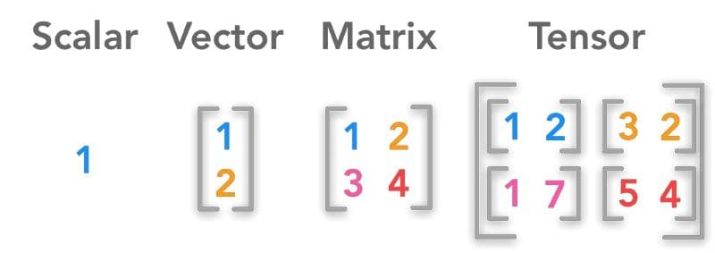
• A scalar (n) is a real number, it is a 0D array and its rank is 0 e.g. 5
• A vector (x) is a 1D array, it has a rank of 1 e.g. [1,2]
• A matrix (X) is a 2D array, that has a rank of 2 e.g. [[1,2], [3,4]]
• A tensor is a general term for 3 or more dimensions array e.g. [ [[1,2], [3,4]], [[5,6,7], [8,9,10]] ]

Vectors

A vector is a quantity that has both magnitude and direction, it can be represented as a list of numbers, given in small letters as $v_1, v_2, ..., v_n$. Two equal length vectors $a = [1,2], b = [3,4]$ can be added, subtracted, multiplied and divided as $c = a + b$, where $c[1] = a[1] + b[1]$ to give $c = [4,6]$.

We can calculate the sum of the multiplied elements of two vectors called the dot product. In general, for vectors $a, b \in R^n$, the inner product is $a'b := \sum_{i=1}^n a_i b_i$. In this case, $a.b = (1 \times 3 + 2 \times 4) = 11$.

Two vectors given as columnar matrices $u_m, v_n$, can be multiplied to produce a matrix $A_{mn}$. The outer product of two vectors $u \otimes v = uv^T = A$. Let $u = \begin{bmatrix} u_1 \\ u_2 \end{bmatrix} \; and \; v = \begin{bmatrix} v_1 \\ v_2 \\ v_3 \end{bmatrix}$, the outer product is given by $uv^T = \begin{bmatrix} u_1 \\ u_2 \end{bmatrix} \begin{bmatrix} v_1 & v_2 & v_3 \end{bmatrix} = \begin{bmatrix} u_1 v_1 & u_1 v_2 & u_1 v_3 \\ u_2 v_1 & u_2 v_2 & u_2 v_3 \end{bmatrix}$.

Vectors can also be multiplied by real numbers or quantities that have a magnitude only called scalars. A number $\gamma = 5$ can be multiplied by the vector $a$ such that $\gamma a = \begin{bmatrix} \gamma a_1 \\ \gamma a_2 \end{bmatrix}$ to give $[5,10]$.

Linear Combination and Independence

A Linear combination of two or more vectors is a vector obtained from the sum of the vectors multiplied by scalar values. Given two vectors $v_1 = (2,3) \: and \: v_2 = (4,5)$, we can get $v_3 = c_1v_1 + c_2v_2$, for scalar values $c_1 =2 \: and \: c_2=3$.

$c_1v_1 + c_2v_2 = 2 \begin{bmatrix} 2 \\ 3 \end{bmatrix} + 3 \begin{bmatrix} 4 \\ 5 \end{bmatrix} = \begin{bmatrix} 2 \times 2 + 3 \times 4 \\ 2 \times 3 + 3 \times 5 \end{bmatrix} = \begin{bmatrix} 16 \\ 21 \end{bmatrix}$

Given $v_1, v_2$ and the linear combination $v_3$, we can get the scalar multiples using the RREF (move towards an identity matrix by swapping, multipling and adding rows).

$\begin{bmatrix} v_1 & v_2 & | & v_3 \\ 2 & 4 & | & 16 \\ 3 & 5 & | & 21 \end{bmatrix}$. By (R2 - R1), (-3R1+R2), and (R2/2), we get $\begin{bmatrix} c_1 & c_2 & & \\ 1 & 1 & | & 5 \\ 0 & 1 & | & 3 \end{bmatrix}$. Since $c_2 = 3$, $c_1 + 3 = 5$, thus $c_1 =2$.

Vectors are linear independent if none of them can be expressed as a linear combination of the others. In this case $c_1v_1 + c_2v_2 = 0 = (0,0)$, with $c_1 = c_2 = 0$. If the only way to to get $0 = \sum_{i=1}^{k}c_{i}v_{i}$ requires all $c_1,...,c_k = 0$, we have linearly independent vectors. To find if a = (1,3) and b = (2,5) are linear independent.

$\begin{bmatrix} a & b & | & \\ 1 & 2 & | & 0 \\ 3 & 5 & | & 0 \end{bmatrix}$. By (-3R1+ R2), $\begin{bmatrix} c_1 & c_2 & | & \\ 1 & 2 & | & 0 \\ 0 & 1 & | & 0 \end{bmatrix}$. Since $c_2 = 0$ and $c_1 = 0$, the two vectors are linearly independent.

Vector space

A vector space is a set of vectors and all their possible combinations. Elements of $R^n$ are a set of real numbers, such as $x = \begin{bmatrix} 1 \\2 \end{bmatrix} = \begin{bmatrix}x_1 \\ x_2 \end{bmatrix} \in \mathbb R^2$. Given a set of vectors $V = \begin{Bmatrix} \begin{bmatrix} 0 \\ 1 \end{bmatrix}, \begin{bmatrix} 1 \\ 0 \end{bmatrix} \end{Bmatrix}$, the span is the subspace composed of all possible linear combinations of the vectors in that set, which is $R^2$. The standard basis $\begin{Bmatrix} \begin{bmatrix} 0 \\ 1 \end{bmatrix}, \begin{bmatrix} 1 \\ 0 \end{bmatrix} \end{Bmatrix}$, can write every vector in $R^2$ for example, $\begin{bmatrix} a \\ b \end{bmatrix} = a \cdot \begin{bmatrix} 1 \\ 0 \end{bmatrix} + b \cdot \begin{bmatrix} 0 \\ 1 \end{bmatrix}$. In general, given $V = \begin{Bmatrix} v_1, v_2, ..., v_3 \end{Bmatrix}, \; the \; span(V) = \alpha v_1 + \alpha v_2 + ... + \alpha v_n$.

Another set $\begin{Bmatrix} \begin{bmatrix} 0 \\ 1 \end{bmatrix}, \begin{bmatrix} 1 \\ 0 \end{bmatrix}, \begin{bmatrix} 2 \\ 0 \end{bmatrix} \end{Bmatrix}$ is a spanning set of $R^2$ but not a basis for $R^2$ . Having both (1,0) and (2,0) in the set creates linear dependence, thus cannot be a basis for $R^2$.

Finding the basis of a subspace

Given $V = Span \begin{Bmatrix} \begin{pmatrix} 1 \\ 0 \end{pmatrix}, \begin{pmatrix} 3 \\ 1 \end{pmatrix}, \begin{pmatrix} -1 \\ 7 \end{pmatrix} \end{Bmatrix}$, the subspace V is the column matrix of the matrix $A = \begin{pmatrix} 1 & 3 & -1 \\ 0 & 1 & 7 \end{pmatrix}$. The reduced echelon is $\begin{pmatrix} 1 & 0 & -22 \\ 0 & 1 & 7 \end{pmatrix}$. The first two columns are pivot columns, the basis V is $\begin{Bmatrix} \begin{pmatrix} 1 \\ 0 \end{pmatrix}, \begin{pmatrix} 3 \\ 1 \end{pmatrix} \end{Bmatrix}$. The number of linearly independent columns of a matrix is the rank of the matrix.

Decomposition of a vector by the basis vectors

Decompose vector $b = \begin{pmatrix} 10,30 \end{pmatrix}$ by basis vectors $p = \begin{pmatrix} 2, 2 \end{pmatrix} \; and \; q = \begin{pmatrix} -1, 4 \end{pmatrix}$.

We use the coefficients for x, y to form the equation $\vec{xp} + \vec{yq} = \vec{b}$, that is $\begin{cases} 2x - y = 10 \\ 2x + 4y = 30 \end{cases}$. The $x = -1, y = 3$, we conclude that $\vec {b} = \vec{-p} + \vec{3q}$.

Angle between two vectors

Given two vectors $\vec{a}= \begin{pmatrix}-3, 4 \end{pmatrix}, \vec{b} = \begin{pmatrix}{5, 12} \end{pmatrix}$, we can find the angle between them.

Orthogonal basis

A basis $V = \begin{Bmatrix} v_{1}, v_{2} \end{Bmatrix}$ is orthogonal if the vectors that form it are perpendicular $\begin{pmatrix}90^0 \end{pmatrix}$, their dot product is zero. Given $v_1 = \begin{Bmatrix}4;-2 \end{Bmatrix}, v_2 = \begin{Bmatrix}5;10 \end{Bmatrix}$, then $v_1 \cdot v_2 = 4 \cdot 5 + (-2) \cdot 10 = 0$;

In cases where the dot product is zero (0) and the length of each vector is one (1), it is called orthonormal basis. Given $v_1 = \begin{Bmatrix}1;0 \end{Bmatrix}, v_2 = \begin{Bmatrix}0;-1 \end{Bmatrix}$, then $v_1 \cdot v_2 = 1 \cdot 0 + 0 \cdot (-1) = 0$. In addition, the lengths of $|\vec{v_1}| = \sqrt{ 1^2 + 0^2} = 1 \; and \; |\vec{v_2}| = \sqrt{0^2 + (-1)^2} = 1$.

Vector norm (length/magnitude)

For $p \ge 1$ the p-norm of $v = \begin{pmatrix} v_1,...,v_n \end{pmatrix}$ is $\| x \|_{p} := \begin{pmatrix} \sum_{i=1}^{n} |x_i|^p \end{pmatrix}^{1/p}$

• $l^1$-norm also called the taxicab/manhattan distance which is a sum of the absolute value of vector elements, the p = 1. Given $v = [1,2,3]$ then $||v||_1 = 1+2+3 = 6$.
• $l^2$-norm also called the Euclidean distance is a straight line, the p = 2. Given $v = [1,2,3]$ , then $||v||_2 = \sqrt{1^2 + 2^2 + 3^2} = 3.74$.
• $l^{inf}$-norm also called the Chebyshev/max distance is the maximum value. Given $v = [1,2,3]$, then $||v||_{inf} = max(1,2,3) = 3$.

Cross Product

Two vectors can be multiplied to produce another vector that is perpendicular to both of the two vectors. In general, with $a = (x, y, z) \; and \; b = (x, y, z)$, the new vector $c = (a_y \cdot b_z - a_z \cdot b_y, a_z \cdot b_x - a_x \cdot b_z, a_x \cdot b_y - a_y \cdot b_x)$. Given $(1,2,3) \times (4,5,6) = (2*6 - 3*5, 3*4 - 1*6, 1*5 - 2*4) = (-3,6,-3)$.

Matrices

A matrix is a rectangular array of numbers arranged into columns and rows. The matrix A has m rows and n columns. Each entry of A becomes $a_{ij}, \; where \; i=1...m$ and $j=1...n$. For a matrix $A \in \mathbb R^{m \times n}$, then

$A := \begin{bmatrix}a_{11} & \cdots & a_{1n} \\ \vdots & \cdots & \vdots \\ a_{m1} & \cdots & a_{mn} \end{bmatrix}, a_{ij} \in \mathbb R$.

Zero Matrix

A null matrix, has a zero in all entries.

def zeros_matrix(i=None, j=None):
    """
    A matrix filled with zeros.
    
    params:
        i : number of rows
        j: number of columns
    return: list of lists
    
    """
    
    if j == None:
        j = i
        
    M=[]
    #Create rows
    while len(M) < i:
        M.append([])
        #Enter values for each row 
        while len(M[-1]) < j:
            M[-1].append(0)
    return M

In []: zeros_matrix(3)

Out []: [[0, 0, 0], [0, 0, 0], [0, 0, 0]]

Identity Matrix

It is a square matrix in which all elements of the principal diagonal running from upper left to lower right are ones and all other elements are zero.

def eye(n=None):
    """
    Create an identity matrix for a square matrix
    shorter method: [[float(i==j) for i in range(n)] for j in range(n)]
    params
        n: number of rows and columns
    return: list of lists   
    """
    
    if (n == None):
        matrix = []
    else:
        matrix = zeros_matrix(n)
    for i in range(n):
        matrix[i][i] = 1
    return matrix  

In []: eye(3)

Out []: [[1, 0, 0], [0, 1, 0], [0, 0, 1]]

Copying a Matrix

To prevent unexpected bugs, it is a good practice to make a copy of a matrix before using it.

def copy_matrix(M):
    """
    Creates a copy of the matrix provided
    params: 
        M: a matrix / list of lists
    return: A list of lists
    """
    NM = []
    for i in range(len(M)):
        temp = []
        for j in range(len(M[0])):
            temp.append(M[i][j])
        NM.append(temp)
        
    return NM

def test_matrix(M):
	for x in range(len(M)):
		M[x][x] = 1.0
	return M

matrix = [[0]*2]*2    
cmatrix = copy_matrix(matrix)

In []: test_matrix(matrix)  #python 3.7
Out []: [[1,1],[1,1]]
In []: test_matrix(cmatrix)
Out []: [[1,0],[0,1]]

Matrix Transformation

Matrix Addition

Matrices of the same shape can be added together $A_{ij} + B_{ij} = C_{ij}$. The sum of $A \in \mathbb R^{m \times n}$ and $B \in \mathbb R{m \times n}$ is given by:

$A + B = \begin{bmatrix} a_{11} + b_{11} \cdots a_{1n} + b_{1n} \\ \vdots \ddots \vdots \\ a_{m1} + b_{m1} \cdots a_{mn} + b_{mn} \end{bmatrix}$

def shape(M=None):
    """
    Give the size i.e. the number of rows and columns
    params: 
        M: A matrix that has rows and columns
    return: a list containing [rows,columns]
    """
    return [len(M), len(M[0])]

def matrix_addition(MA,MB):
    """
    Add two matrices of the same shape
    params: 
        MA: a matrix
        MB: a matrix
        
    return: matrix
    """
    A = copy_matrix(MA)
    B = copy_matrix(MB)

    if shape(A) != shape(B):
        raise ArithmeticError("Matrices are not of the same size.")
        
    C = [];
    for i in range(len(A)):
        row_vals = []
        for j in range(len(B[0])):
            if ( type(A[i][j]) == int or type(A[i][j]) == float) and ( type(B[i][j]) == int or type(B[i][j]) == float):
            	#For matrix subtraction change sign to (-)
                row_vals.append(A[i][j] + B[i][j])
            else: 
                raise TypeError("All Matrix values must be numbers.")
        C.append(row_vals)
    return C

In []: matrix_addition([[1,2],[2,3]], [[4,5],[6,7]])
Out []: [[5,7,],[8,10]]

Given two matrices $A_{23} = \begin{bmatrix}1 & 2 & 3 \\ 4 & 5 & 6 \end{bmatrix} \; and \; B_{22} = \begin{bmatrix} 7 & 8 \\ 9 & 10 \end{bmatrix}$ of unequal dimensions, we can get their direct sum as follows:

Matrix Multiplication

Matrix $A$ can be multiplied by a scalar value $\alpha$ to give $\alpha (A_{ij})$. $A$ can also be multiplied (dot product) by a matrix $B$ as long as the columns of $A$ are equal to the rows $B$.

$c_{ij} := \sum{l=1}^n a_{il} b{lj}$

• Associativity : A(BC) = (AB)C
• Not Commutative : $A \dot B \neq B \dot A$

In hardamard product, we multiply two square matrices similar to addition (A * B).

def matrix_multiply(MA, MB):
    """
    Multiply two matrices (dot product), Aij X Bmn => j == m
    shorter method: [[sum((av * bv) for av, bv in zip(a, b)) for b in zip(*MB)] for a in MA ]
    params: 
        MA: a matrix
        MB: a matrix
    return: matrix
    """
    A = copy_matrix(MA)
    B = copy_matrix(MB)

    if not shape(A)[1] == shape(B)[0]:
        raise TypeError("Columns of A are not equal to rows of B")
        
    new_matrix = []
    for i in range(len(A)):
        cols_vals = []
        for n in range(len(B[0])):            
            s = 0
            for m in range(len(B)):
                s += A[i][m] * B[m][n]                
            cols_vals.append(s)            
        new_matrix.append(cols_vals)
        
    #new_matrix(i*n) 
    return new_matrix   
    

In []: matrix_multiply([[1,2],[4,5]], [[7],[9]])
Out []: [[25], [73]]

Determinants

The determinant of a matrix is the multiplicative change from tranforming a space with the matrix. We check the determinant while looking for an inverse of a square matrix. A square matrix that has a determinant of zero is singular and it has no inverse. For a matrix $A_{22}= \begin{bmatrix} a_{11} & a_{12} \\ a_{21} & a_{22} \end{bmatrix}$ the determinant $|A| = a_{11}.a_{22} - a_{12}.a_{21}$. In matrices larger than 2x2, we use cofactor expansion to get the determinants.

def recursive_determinant(RM, multi=1):
        """
        The determinant of a square matrix using cofactor
        Cofactor is created by an element of a matrix e.g. m[0][1] when it excludes m[i][1] and m[0][j]
        params:
            RM: a matrix/ list of lists
            multi: a multiplier number
        returns: the total for the levels of recursion
        """
        
        width = len(RM)
        if width == 1:
            return multi * RM[0][0]
        else:
            sign = -1
            total = 0
        #Starts here
        for i in range(width):
            m = []
            #loop removes first row and exclude values from the ith column all the way down till we have 1 row, select the kth
            #multi is the (ith) matrix[0][i] before the last 2 rows, sign*matrix[0][i]: ith value when two rows are remaining
            #m is kth value when only 1 row remains
            for j in range(1, width):
                temp = []
                for k in range(width):
                    if k != i:
                        temp.append(RM[j][k])  
                m.append(temp)
                
            sign *= -1            
            total += multi * recursive_determinant(m, sign * RM[0][i])
            
        return total

In []: rmx = [[5,2,3,16],[5,6,7,8],[9,10,11,12],[13,14,15,4]]
In []: recursive_determinant(rmx)
Out []: 192

There is a faster way of finding the determinant by reducing the square matrix into an upper triangle matrix as explained here.

def faster_determinant(MF):
	"""
	The upper triangle method.

	params: 
		A: a square matrix
	return: a number
	"""
	matrix = copy_matrix(MF)

    n = len(matrix)
    
    for d in range(n):
        for i in range(d+1, n):
            if matrix[d][d] == 0:
                matrix[d][d] = 1.8e-18
                
            row_scaler = matrix[i][d] / matrix[d][d]
    
            for j in range(n):
                matrix[i][j] = matrix[i][j] - row_scaler * matrix[d][j]
    
    
    product = 1.0
    
    #determinant is the product of diagonals
    for i in range(n):
        product *= matrix[i][i]
    return product

In []: rmx = [[5,2,3,16],[5,6,7,8],[9,10,11,12],[13,14,15,4]]
In []: faster_determinant(rmx)
Out []: 192

Inverse of a matrix

Similar to an inverse of a number ($5 \times 1/5 = 1$), an inverse of a matrix multiplied by the matrix yields 1. The inverse of a matrix will satisfy the equation $A (A^{^-1}) = I$. For a matrix to be invertible, it must be a square and its determinant must not be zero.

def matrix_inverse(M):
    """
    Find inverse by transforming the matrix into an identity matrix:
        1. Scale the each row by its diagonal value
        2. Subtract (diagonal column value * diagonal row values) from each row except the diagonal row
    params: 
        A: a square matrix
    return a matrix
    """
   
    n = len(M)
    IM = eye(n)
    
    matrix = copy_matrix(M)
    imatrix = copy_matrix(IM)
    
    
    assert shape(matrix)[0] == shape(matrix)[1], "Make sure the matrix is squared"
    assert faster_determinant(matrix) != 0, "The matrix is singular, it has no inverse."
   
    indices = list(range(n))
    for d in range(n):
        ds = 1.0 / matrix[d][d]
        #diagonal scaler 
        for j in range(n): 
            matrix[d][j] *= ds
            imatrix[d][j] *= ds
    
        #row scaler    
        for i in range(n):
            if i != d:
                rs = matrix[i][d]  
                for j in range(n):
                    matrix[i][j] = matrix[i][j] - rs * matrix[d][j]
                    imatrix[i][j] = imatrix[i][j] - rs * imatrix[d][j]
    return imatrix

In []: aa= [[3,7],[2,5]]
In []: matrix_inverse(aa)
Out []: [[ 5., -7.],[-2.,  3.]]

Matrix Division

To divide matrices we multiply them by an inverse. Lets consider $A \div B$ where as $A_{2X2} = \begin{bmatrix} 13 & 26 \\ 39 & 13 \end{bmatrix}$ and $B_{2X2} = \begin{bmatrix} 7 & 4 \\ 2 & 3 \end{bmatrix}$. To find $A \times B'$;

In []: A = [[13,26],[39,13]]
In []: B_inv = matrix_inverse([[7,4],[2,3]])
In []: matrix_multiply(A, B_inv)
Out []: [[-1,10],[7,-5]]

Solving a System of Linear Equations

The matrix solution is represented as $Ax = b$, therefore $x = bA'$.

1. $5a + 3b + 7c = 74$
2. $9a + 2b + 6c = 73$
3. $4a + 2b + 5c = 53$

In []: A_inv = matrix_inverse([[5,3,7],[9,2,6],[4,2,5]])
In []: matrix_multiply(A_inv, [[74], [73], [53]])
Out []: [[3.0], [8.0], [5.0]]

Transpose

We pivot matrices to enable multiplication and division, this is done by switching columns by rows $A_{ij} = A_{ji}^T$. From $A_{3X2} = \begin{bmatrix} a_{11} & a_{12} \\ a_{21} & a_{22} \\ a_{31} & a_{31} \end{bmatrix}$ to $A^T_{2X3} = \begin{bmatrix} a_{11} & a_{12} & a_{13} \\ a_{21} & a_{22} & a_{23} \end{bmatrix}$.

def transpose(MT=None):
    """
    Create a transpose of a matrix ( Mij =>  Mji)
    shorter method: [list(x) for x in  zip(*MT)]
    params:
        matrix : a value, list or list of lists
    return: list of lists
    """
    matrix = copy_matrix(MT)

    if matrix == None:
        matrix = [[]]
    elif not isinstance(matrix, list):
        matrix = [[matrix]]
    elif not isinstance(matrix[0], list):
        matrix = [matrix]
    
    new_matrix = []
    for j in range(len(matrix[0])):
        new_vals = []
        
        for i in range(len(matrix)):
            new_vals.append(matrix[i][j])
        new_matrix.append(new_vals)
        
    return new_matrix

In []: transpose([1,2])
Out []: [[1],[2]]

In []: tranpose([[1,2,3],[4,5,6]])
Out []: [[1,4],[2,5],[3,6]]

Special Matrices

Square Matrix

$\begin{bmatrix} 1 & 2 & 3 \\ 4 & 5 & 6 \\ 7 & 8 & 9 \end{bmatrix}$

Rectangular Matrix

$\begin{bmatrix} 1 & 2 & 3 \\ 4 & 5 & 6 \end{bmatrix}$

Diagonal Matrix

$\begin{bmatrix} 3 & 0 & 0 \\ 0 & 4 & 0 \\ 0 & 0 & 5 \end{bmatrix}$

Anti-diagonal Matrix

$\begin{bmatrix} 0 & 0 & 3 \\ 0 & 4 & 0 \\ 5 & 0 & 0 \end{bmatrix}$

Symmetric Matrix

$\begin{bmatrix} 1 & 2 & 3 \\ 2 & 1 & 5 \\ 3 & 5 & 1 \end{bmatrix}$

Scalar Matrix

$\begin{bmatrix} 2 & 0 & 0 \\ 0 & 2 & 0 \\ 0 & 0 & 2 \end{bmatrix}$

Pivoting

In Gaussian elimination, the pivot element is required to not be zero. Given $\begin{bmatrix}1 & 2 & 3 \\ 4 & 0 & 5 \\ 6 & 7 & 8 \end{bmatrix}$, we swap to produce $\begin{bmatrix}1 & 2 & 3 \\ 6 & 7 & 8 \\ 4 & 0 & 5 \end{bmatrix}$. It is also desired to have the pivot element with a large absolute value to reduce the effect of rounding off error. Given $\begin{bmatrix}0.003 & 59.14 \\ 5.291 & -6.13 \end{bmatrix}$, after swapping we get $\begin{bmatrix}5.291 & -6.13 \\ 0.003 & 59.14 \end{bmatrix}$. In a partial pivot, we select the entry with the largest absolute value from the column of the matrix that is currently being considered as the pivot element.

def pivot(m):
    """
    Rearrange row values, the larger value becomes the pivot element 
    params:
        m: matrix
    returns: a matrix containing 0,1's
    """
    n = len(m)
    Id = [[float(i==j) for i in range(n)] for j in range(n)]
    #get the max value in each, if not at pivot position, swap.
    for j in range(n):
        row = max( range(j, n), key=lambda i: abs(m[i][j]) )
     
        if j != row:
            Id[j], Id[row] = Id[row], Id[j]
    return Id

In []: vals = [[5,3,8],[6,4,5],[2,11,9]]

In []: pivot(vals)
Out []: [[0,1,0],[0,0,1],[1,0,0]]

In []: matrix_multiply(vals, pivot(vals))
Out []: [[8,5,3],[5,6,4],[9,2,11]]

MATRIX FACTORIZATION

Matrix decompositions reduce a matrix into constituent parts that make it easier to do complex operations. They can be used to calculate determinants, inverse and in solving systems of linear equations.

Lower and Upper Triangle Matrix Decomposition (LU)

A non-singular square matrix is decomposed in the form $A = L.U$. To prevent division by zero error we pivot, such that $PA = LU$.

LU decomposition using Crout's algorithm

The diagonals of a U matrix in Crout decomposition are 1, in Doolittle algorithm the diagonals of L matrix are all 1.

To calculate the upper values:

We derive the formula for U

To calculate the lower values:

We derive the formula for L

def lup(M):
    """
    Perform a Lower and Upper Decomposition.
    params:
        M: a nxn matrix
    return: 3 nxn matrices; Lower, Upper and Pivot.
    """
    n = len(M)
    L = [[0.0]*n for i in range(n)]
    U = [[0.0]*n for i in range(n)]
    P = pivot(M)
    PM = matrix_multiply(P,M)
    for j in range(n):
        L[j][j] = 1.0
        
        for i in range(j+1):
            s1 = sum(U[k][j] * L[i][k] for k in range(i))
            U[i][j] = PM[i][j] - s1
        for i in range(j, n):
            s2 = sum(U[k][j] * L[i][k] for k in range(j))
            L[i][j] = (PM[i][j] - s2) / U[j][j]
    return L,U,P

In []: lup([2,3,5],[2,4,7],[6,8,0]])
Out []: (
	[[1.0,0.0,0.0],[0.3,1.0,0.0],[0.3,4.0,1.0]],  #L
	[[6.0,8.0,0.0],[0.0,0.3,5.0],[0.0,0.0,-13.0]],  #U
	[[0.0,0.0,1.0],[1.0,0.0,0.0],[0.0,1.0,0.0]]     #P
	)

Solving a Linear System using LU decomposition

Given an $L = \begin{bmatrix} 1 & 0.0 & 0.0 \\ 0.3 & 1.0 & 0.0 \\ 0.1 & -0.03 & 1.0 \end{bmatrix}$, $U = \begin{bmatrix} 3.0 & -0.1 & -0.2 \\ 0.0 & 7.0 & -0.3 \\ 0.0 & 0.0 & 10.0 \end{bmatrix}$ and $b = \begin{bmatrix}7.85 \\ -19.3 \\ 71.4 \end{bmatrix}$. The $PA = LU$, P is a permutation matrix that swaps rows of A. A linear system is $Ax = b$, since $A == LU$, then $(LU)x = b$. We can shift the parenthesis such that $L(Ux) = b$, lets create a d such that $Ld = b$. Finally, we find x using $Ux = d$.

Solving for d using forward substitution

def forward_substitution(l, b):
    """
    Calculating the value of d given Ld = b
    params:
        L: a non-singular nxn matrix
        b: a vector
    return: a vector
    """
    n = len(l)
    for i in range(0, n-1):
        for j in range(i+1, n):
            b[j] -= l[j][i] * b[i]
    return b

Solving for x using back substitution

 def back_substitution(u, d):
    """
    Calculating the value of x given Ux = d
    params: 
        U: a non-singular, nxn matrix
        d: a vector
    return: a vector
    """
    n = len(u)
    #the upper matrix is upside down
    #start with the last row and move upwards
    for i in range(n)[::-1]:
        d[i] /= u[i][i]
        for j in range(0, i):
            d[j] -= u[j][i] * d[i]   
    return d

In []: l,u,p = lup([[3,-0.1,-0.2],[0.1,7,-0.3],[0.3,-0.2,10]])
In []: b = [7.85, -19.3, 71.4]
In []: d = forward_substitution(l, b)
In []: back_substitution(u, d)
Out []: [3.0, -2.5, 7.0]  #x1, x2, x3

FURTHER READING

• Integrated Machine Learning
• Introduction to Vectors Matrices and Tensors
• Linear Algebra in Python
• LU Decomposition